PCR and RT-PCR Protocols for Gene Amplification: A Comprehensive Guide from Basics to Advanced Applications

Abstract

This article provides a comprehensive guide to PCR and Reverse Transcription PCR (RT-PCR) protocols, tailored for researchers, scientists, and drug development professionals. It covers foundational principles, distinguishing between key techniques like PCR, qPCR, RT-PCR, and RT-qPCR. The guide delves into detailed, step-by-step methodological protocols for both one-step and two-step RT-PCR, including RNA extraction, reverse transcription, and amplification. It offers extensive troubleshooting and optimization strategies for common challenges such as weak amplification and non-specific products. Finally, it addresses validation and data analysis, emphasizing accurate normalization in quantitative applications to ensure reliable gene expression analysis, viral load detection, and other critical research and diagnostic outcomes.

PCR Fundamentals: Understanding Core Principles and Technique Selection

Polymerase chain reaction (PCR) and its advanced derivatives represent foundational technologies in molecular biology, enabling the detection and analysis of nucleic acids with unparalleled sensitivity. These techniques form the cornerstone of gene amplification research, supporting advancements in drug development, diagnostics, and fundamental biological research. This article provides a detailed technical overview of key PCR methodologies—standard PCR, quantitative PCR (qPCR), reverse transcription PCR (RT-PCR), and quantitative reverse transcription PCR (RT-qPCR)—framed within the context of developing robust experimental protocols for research scientists. We will explore the principles, applications, and specific experimental considerations for each technique, supplemented with structured data comparisons and detailed workflow visualizations to serve as a practical resource for laboratory application.

Core Principles and Techniques

The PCR Family of Methods

At its core, PCR is a method for amplifying a specific segment of DNA through repetitive temperature cycles, achieving exponential replication of the target sequence [1]. The basic mechanism involves three steps per cycle: denaturation of double-stranded DNA, annealing of primers to complementary sequences, and elongation of new DNA strands by a heat-stable DNA polymerase [2]. This process allows researchers to generate billions of copies from a single or few DNA molecules, facilitating downstream analysis.

Table 1: Comparative Overview of Core PCR Techniques

Technique	Template	Key Principle	Detection Method	Primary Applications	Data Output
PCR	DNA	Amplification via thermal cycling	Endpoint, gel electrophoresis	DNA cloning, mutation detection, template generation	Qualitative (Presence/Absence)
qPCR	DNA	Real-time monitoring of amplification	Fluorescence (dye or probe-based)	Gene quantification, pathogen load, SNP genotyping	Quantitative (Absolute/Relative)
RT-PCR	RNA	Reverse transcription to cDNA before amplification	Endpoint, gel electrophoresis	RNA virus detection, cDNA library construction	Qualitative (Presence/Absence)
RT-qPCR	RNA	Reverse transcription followed by real-time quantification	Fluorescence (dye or probe-based)	Gene expression analysis, viral load quantification	Quantitative (Absolute/Relative)

Technical Elaboration of Methods

Standard PCR serves as the foundational technique, where amplification is typically analyzed at the reaction endpoint, most commonly via agarose gel electrophoresis [1] [2]. This method is indispensable for applications requiring DNA detection rather than quantification, such as genotyping, cloning, and sequence verification.

Quantitative PCR (qPCR), also known as real-time PCR, incorporates fluorescent detection systems to monitor DNA accumulation during the exponential phase of amplification [1]. This enables precise quantification of initial template amounts. Two primary detection chemistries are employed:

• Dye-based detection (e.g., SYBR Green): Utilizes fluorescent dyes that intercalate non-specifically into double-stranded DNA [2]. This method is cost-effective but may detect non-specific products like primer-dimers.
• Probe-based detection (e.g., TaqMan, Molecular Beacons): Employs sequence-specific oligonucleotide probes labeled with fluorophores and quenchers, offering greater specificity and enabling multiplexing [1] [2].

Reverse Transcription PCR (RT-PCR) is designed for RNA detection by first converting RNA to complementary DNA (cDNA) using a reverse transcriptase enzyme [1] [3]. This cDNA then serves as the template for standard PCR amplification. The quality of the RNA template and the efficiency of the reverse transcription reaction are critical factors for success [1].

Quantitative Reverse Transcription PCR (RT-qPCR) combines the RNA-to-cDNA conversion of RT-PCR with the quantitative capabilities of qPCR [2]. This powerful technique is the gold standard for quantifying RNA transcripts, enabling applications such as gene expression analysis under different experimental conditions and precise measurement of viral RNA loads [1].

Experimental Protocols and Applications

Detailed Protocol: Primer Design and Validation for Specific Detection

Accurate detection of target organisms in complex samples requires carefully designed and validated primers. The following protocol, adapted from studies on Listeria and Pseudomonas aeruginosa detection, outlines a robust workflow for species-specific primer development [4] [5].

Objective: To design and validate species-specific primers for accurate detection of target sequences in bacterial cultures and food samples.

Materials:

• Software: Geneious, PrimerSelect, or equivalent primer design software; BLAST database access [4]
• Template DNA: Genomic DNA from target and non-target reference strains [4]
• PCR Reagents: Thermostable DNA polymerase (e.g., Taq, Ex Taq), corresponding reaction buffer, dNTPs, nuclease-free water [4]
• Equipment: Thermal cycler, qPCR instrument (e.g., for SYBR Green chemistry), agarose gel electrophoresis system [4]

Procedure:

• Target Gene Selection: Perform comparative genomic analysis of target and non-target strains to identify unique, conserved gene regions. For L. monocytogenes and L. innocua differentiation, target genes encoding a hypothetical protein with an LPXTG cell wall anchor domain and leucine-rich repeats were identified, respectively [4].
• In Silico Primer Design:
  • Design primers with length of 18-22 bp, GC content of 40-60%, and melting temperature (Tm) of 55-65°C.
  • Avoid self-complementarity and secondary structures.
  • Verify specificity in silico using BLASTn against non-redundant databases to ensure no significant homology with non-target species [4].
• Specificity Validation via Conventional PCR:
  • Prepare PCR master mix: 1X reaction buffer, 0.25 mM each dNTP, 10 pM each primer, 1.25 units DNA polymerase, and 5 ng/µL template DNA.
  • Perform amplification: Initial denaturation at 95°C for 5 min; 35 cycles of 95°C for 30s, annealing at 55°C for 30s, 72°C for 30s; final extension at 72°C for 5 min [4].
  • Analyze 5 µL of PCR product by 1.5% agarose gel electrophoresis. Specific amplification should yield a single band of expected size only with target DNA [4].
• Sensitivity and Quantification Validation via qPCR:
  • Prepare standard curves using serial dilutions of different templates: cloned target DNA (positive control), genomic DNA, and bacterial cell suspensions [4] [5].
  • Perform qPCR with appropriate fluorescence detection (e.g., SYBR Green).
  • Assess assay performance: amplification efficiency (>90%), linearity (R² > 0.980), and dynamic range [4] [6].
• Application Testing: Validate primer performance in actual sample matrices (e.g., inoculated food samples like mushrooms or carrots) to confirm detection accuracy in complex backgrounds [4] [5].

Detailed Protocol: RT-qPCR for Gene Expression Analysis

RT-qPCR is the method of choice for precise quantification of gene expression levels. Adherence to the MIQE (Minimum Information for Publication of Quantitative Real-Time PCR Experiments) guidelines is essential for generating reproducible and reliable data [7] [8].

Objective: To accurately quantify relative or absolute changes in mRNA expression levels between samples.

Materials:

• RNA Sample: High-quality, intact total RNA or mRNA [1]
• Reverse Transcriptase: RNase H- reduced enzymes (e.g., M-MLV, ProtoScript II) for improved full-length cDNA synthesis [3]
• qPCR Reagents: qPCR master mix, sequence-specific primers, and probe (if using probe-based chemistry) or fluorescent DNA-binding dye (e.g., SYBR Green) [2]
• Equipment: Thermal cycler, real-time PCR instrument [4]

Procedure:

• RNA Extraction and Quality Control: Extract RNA using a method that minimizes RNase contamination. Assess RNA integrity and purity using spectrophotometry (A260/A280 ratio ~1.8-2.0) and/or agarose gel electrophoresis [1].
• Reverse Transcription (cDNA Synthesis):
  • In a nuclease-free tube, combine 1 µg of total RNA, reverse transcriptase (e.g., 1 µL of 200 U/µL ProtoScript II), appropriate reaction buffer, dNTPs (0.5 mM each), and oligo(dT) or random hexamer primers [3].
  • Incubate at 42-50°C for 30-60 minutes, followed by enzyme inactivation at 85°C for 5 min. The higher temperature capability of engineered reverse transcriptases helps overcome RNA secondary structures [3].
• qPCR Assay Setup:
  • Prepare reactions containing diluted cDNA template, 1X qPCR master mix, and gene-specific primers. Include no-template controls (NTC) for each primer set.
  • For absolute quantification, include a standard curve of known template copy numbers [7].
• qPCR Amplification:
  • Program the thermal cycler: initial denaturation (95°C, 5 min); 40 cycles of denaturation (95°C, 15-30s), annealing (primer-specific Tm, 30s), and extension (72°C, 30s); with fluorescence acquisition at each cycle's end [4].
• Data Analysis:
  • Determine Cq (quantification cycle) values for each reaction.
  • For relative quantification, normalize target gene Cq values to reference gene(s) (e.g., GAPDH, β-actin) and calculate relative expression using methods like 2^(-ΔΔCq) [7].
  • Report results with efficiency-corrected target quantities, detection limits, and dynamic ranges per MIQE guidelines [8].

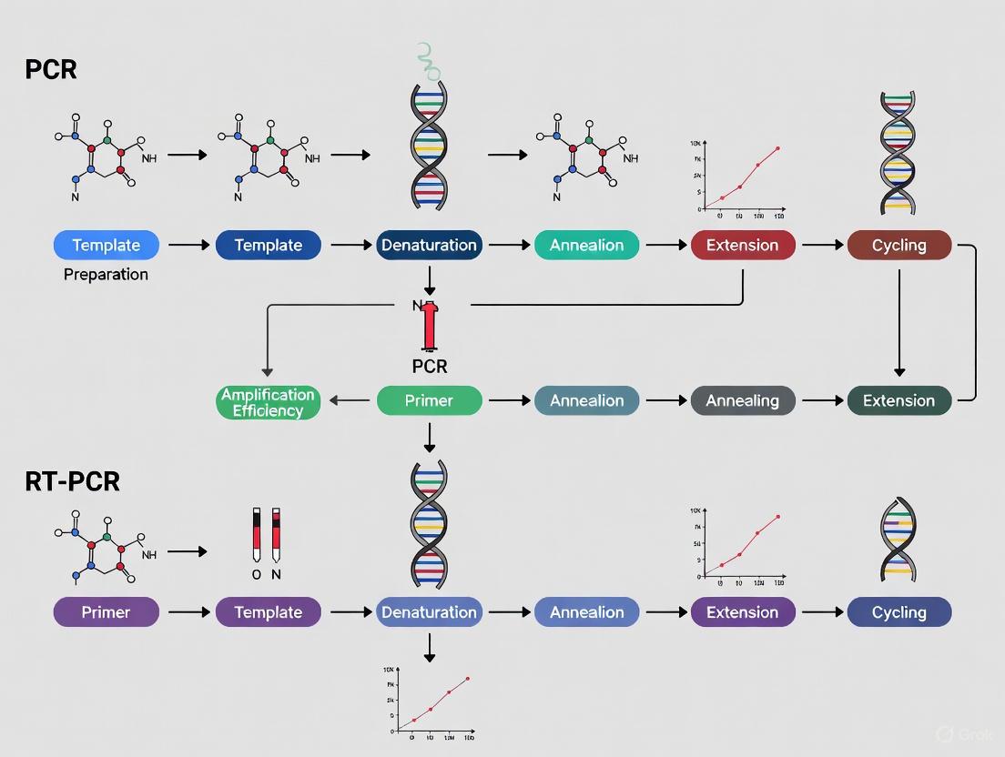
Workflow Visualization

The Scientist's Toolkit: Essential Research Reagents

Table 2: Key Research Reagent Solutions for PCR Applications

Reagent / Material	Function / Purpose	Technical Notes
Hot-Start DNA Polymerase	Reduces non-specific amplification by inhibiting polymerase activity at low temperatures.	Often uses antibody-based inhibition; essential for high-specificity applications [1].
High-Fidelity Polymerase	Provides proofreading activity (3'→5' exonuclease) for accurate DNA amplification.	Pfu polymerase has lower error rate than Taq; critical for cloning and sequencing [1].
Reverse Transcriptase (e.g., M-MLV, AMV)	Synthesizes complementary DNA (cDNA) from RNA templates.	Engineered versions with reduced RNase H activity improve yield of full-length cDNA [3].
SYBR Green Dye	Fluorescent dsDNA-binding dye for qPCR detection.	Cost-effective; requires melt curve analysis to verify specificity [2].
TaqMan Probes	Sequence-specific hydrolysis probes for highly specific qPCR detection.	Fluorophore-Quencher system; enables multiplexing; higher specificity than dye-based methods [1] [2].
GC-Rich Enhancers	Improves amplification efficiency through GC-rich regions and secondary structures.	DMSO, glycerol, or betaine can be added to reaction mixes [1].
MIQE Guidelines	Standardized framework for qPCR experimental design and reporting.	Critical for ensuring experimental reproducibility and data credibility [7] [8].
Doxycycline hyclate	Doxycycline hyclate, MF:C22H29ClN2O10, MW:516.9 g/mol	Chemical Reagent
SCR7	SCR7, MF:C18H14N4OS, MW:334.4 g/mol	Chemical Reagent

The PCR family of techniques provides a versatile and powerful suite of tools for nucleic acid analysis in research and drug development. Understanding the distinct applications, advantages, and technical requirements of PCR, qPCR, RT-PCR, and RT-qPCR enables researchers to select the optimal method for their specific experimental goals. The protocols and guidelines presented here—from primer design and validation to rigorous RT-qPCR execution—provide a foundation for generating reliable, reproducible data. As these technologies continue to evolve with advancements such as digital PCR and isothermal amplification, adherence to established best practices and reporting standards remains paramount for advancing scientific knowledge and ensuring the integrity of research outcomes in gene amplification studies.

The Polymerase Chain Reaction (PCR) is a foundational technique in molecular biology that enables the specific amplification of a target DNA sequence. This process facilitates the generation of millions of copies from a single or few DNA molecules, making it indispensable for applications ranging from basic research to clinical diagnostics and drug development [9]. The core PCR process is both elegant and efficient, relying on the precise repetition of three fundamental temperature-dependent steps: denaturation, annealing, and extension [10] [11]. Mastery of these steps and their parameters is critical for researchers to optimize yield, specificity, and fidelity for any given application. This application note provides a detailed examination of the PCR process, complete with optimized protocols and practical guidelines to ensure success in gene amplification research.

The Three Fundamental Steps of PCR

The amplification power of PCR is achieved through the cyclic repetition of three core steps. The following diagram illustrates the sequential and cyclic nature of this process.

Denaturation

The first step in each PCR cycle is denaturation, which involves heating the reaction mixture to a high temperature, typically between 94°C and 98°C, for 15 seconds to 2 minutes [10] [12]. During this step, the hydrogen bonds holding the complementary strands of the double-stranded DNA template together are broken. This results in the separation of the DNA into two single strands, making the internal sequences accessible for primer binding [10] [11]. The initial denaturation at the beginning of the PCR program is often longer (e.g., 2-3 minutes) to ensure complete separation of all template molecules and, when using hot-start polymerases, to activate the enzyme [10] [12]. Templates with high GC content (>65%) may require longer incubation or higher temperatures for complete denaturation [10].

Annealing

Following denaturation, the reaction temperature is rapidly lowered to a defined annealing temperature, typically between 50°C and 65°C, for 15 to 60 seconds [10] [12]. In this step, the forward and reverse primers—short, single-stranded oligonucleotides designed to be complementary to the sequences flanking the target region—bind (or "anneal") to their respective sites on the single-stranded DNA templates [10] [13]. The annealing temperature is a critical parameter determined by the melting temperature (Tm) of the primers, which is the temperature at which 50% of the primer-DNA duplexes are dissociated [10]. A common starting point is to set the annealing temperature 3-5°C below the calculated Tm of the primers [10]. Specificity is often enhanced by optimizing this temperature; if nonspecific amplification occurs, the temperature can be increased incrementally by 2-3°C [10].

Extension

The final step is extension, during which the temperature is raised to the optimal working temperature for the DNA polymerase, commonly 68°C to 72°C [10] [12]. Using the bound primers as a starting point, the DNA polymerase synthesizes a new DNA strand complementary to the template by sequentially adding free deoxynucleoside triphosphates (dNTPs) from the 5' to the 3' direction [10] [11]. The required extension time is directly proportional to the length of the amplicon and the synthesis rate of the polymerase. For instance, Taq DNA polymerase has an average elongation rate of 1 minute per kilobase (kb) of DNA [10] [12]. For amplicons less than 1 kb, 45-60 seconds is often sufficient [12]. In two-step PCR protocols, the annealing and extension steps are combined into a single incubation, typically at 68°C, which is feasible if the primer Tm is within about 3°C of the extension temperature [10].

PCR Optimization Parameters

Achieving efficient and specific amplification requires careful optimization of reaction components and cycling conditions. The table below summarizes key parameters and their optimal ranges.

Table 1: Key PCR Component Optimization Guidelines

Component	Optimal Range/Value	Considerations & Optimization Tips
Template DNA	Plasmid: 0.1–10 ngGenomic DNA: 5–50 ng (up to 1 µg) [12] [13]	High quality, purified DNA is essential. Higher concentrations increase nonspecific amplification; lower concentrations reduce yield [13] [14].
Primers	0.1–0.5 µM each primer [12] [13]	Primers should be 15–30 nt, with Tm of 55–70°C (within 5°C for a pair) and GC content of 40–60% [13]. Higher concentrations may cause mispriming [13].
MgCl₂	1.5–2.0 mM [12]	Acts as a polymerase cofactor. If [Mg²⁺] is too low, no product forms; if too high, nonspecific products appear. Optimize in 0.5 mM increments [12] [14].
dNTPs	200 µM of each dNTP [12]	All four dNTPs (dATP, dCTP, dGTP, dTTP) should be added in equimolar amounts. Lower concentrations (50-100 µM) can enhance fidelity [12] [13].
DNA Polymerase	0.5–2.0 units per 50 µL reaction [12]	1.25 units of Taq DNA polymerase is often ideal. Excessive enzyme can lead to nonspecific products [12] [13].
Cycle Number	25–35 cycles [10]	Fewer cycles (20-25) are preferred for unbiased amplification (e.g., cloning). Up to 40 cycles may be needed for low-copy targets (>45 cycles is not recommended) [10].

Advanced Optimization: Thermal Cycling Parameters

Beyond component concentrations, the thermal cycling profile itself must be optimized. The following table provides standard and advanced parameters for routine and challenging amplifications.

Table 2: PCR Thermal Cycling Parameter Optimization

Step	Standard Protocol	Challenging Templates (GC-rich, Long Amplicons)
Initial Denaturation	95°C for 2–3 minutes [12]	98°C for 2–3 minutes; or longer initial denaturation (up to 5 min) for GC-rich DNA [10].
Denaturation (Cycling)	95°C for 15–30 seconds [12]	98°C for 20–30 seconds [10].
Annealing (Cycling)	5°C below primer Tm, 15–30 seconds [12]	Use a gradient to determine optimal temperature. Can use specialized buffers allowing universal annealing at 60°C [10].
Extension (Cycling)	68–72°C, 1 min/kb for Taq [10] [12]	68–72°C, 2 min/kb for slower polymerases (e.g., Pfu). Longer times for products >3 kb [10] [12].
Final Extension	72°C for 5 minutes [12]	72°C for 10–15 minutes to ensure all products are fully extended and for dA-tailing if cloning [10].

Experimental Protocol: Standard PCR with Taq DNA Polymerase

This protocol is adapted from established guidelines for routine amplification of a 0.5–2.0 kb fragment from a plasmid or genomic DNA template using Taq DNA Polymerase [12].

Research Reagent Solutions

Table 3: Essential Reagents for Standard PCR

Reagent	Function	Example & Final Concentration
Thermostable DNA Polymerase	Enzyme that synthesizes new DNA strands.	Taq DNA Polymerase, 1.25 units/50 µL [12].
10X Reaction Buffer	Provides optimal pH and salt conditions for the reaction.	Typically supplied with enzyme, contains Tris-HCl, KCl, (NHâ‚„)â‚‚SOâ‚„ [12].
MgClâ‚‚ Solution	Essential cofactor for DNA polymerase activity.	1.5-2.0 mM final concentration (often included in buffer) [12].
dNTP Mix	Building blocks (A, T, C, G) for new DNA synthesis.	200 µM of each dNTP [12].
Forward & Reverse Primers	Short sequences that define the start and end of the target amplicon.	0.1–0.5 µM each, designed per guidelines in Table 1 [13].
Nuclease-Free Water	Solvent to bring the reaction to volume.	N/A
Template DNA	The DNA containing the target sequence to be amplified.	0.1–10 ng (plasmid) or 5–50 ng (genomic DNA) [12] [13].

Step-by-Step Procedure

• Reaction Setup (on ice):

  • Assemble the following components in a sterile, thin-walled PCR tube in the order listed to a final volume of 50 µL:
    • Nuclease-free water: to 50 µL final volume
    • 10X PCR Reaction Buffer: 5 µL
    • 10 mM dNTP Mix: 1 µL (200 µM final each)
    • 50 mM MgClâ‚‚: X µL (1.5-2.0 mM final; volume depends on buffer composition)
    • 10 µM Forward Primer: 0.5–2.5 µL (0.1–0.5 µM final)
    • 10 µM Reverse Primer: 0.5–2.5 µL (0.1–0.5 µM final)
    • Template DNA: Y µL (mass as specified in Table 1)
    • Taq DNA Polymerase: 0.25–0.5 µL (1.25 units is a typical start) [12]
  • Mix the contents gently by pipetting and briefly centrifuge to collect the reaction at the bottom of the tube.

• Thermal Cycling:

  • Place the tubes in a preheated thermal cycler and run the following program:
    • Initial Denaturation: 95°C for 2 minutes [12]
    • 25–35 Cycles of:
      • Denaturation: 95°C for 15–30 seconds
      • Annealing: 50–60°C (optimize based on primer Tm) for 15–30 seconds
      • Extension: 68°C for 1 minute per kb of amplicon (e.g., 45 seconds for a 500 bp fragment) [12]
    • Final Extension: 68°C for 5–10 minutes [10] [12]
    • Final Hold: 4–10°C ∞

• Post-Amplification Analysis:

  • Analyze the PCR product by standard agarose gel electrophoresis. A single, sharp band of the expected size should be visible under UV transillumination.

The PCR process, built upon the elegant repetition of denaturation, annealing, and extension, is a powerful tool in the molecular biologist's arsenal. Successful amplification is not merely a function of executing these steps but relies on the meticulous optimization of reaction components and cycling parameters as detailed in this note. By understanding the role and optimal ranges for each reagent and temperature step, researchers can systematically troubleshoot and refine their protocols to achieve high specificity and yield for even the most challenging templates. The provided guidelines and protocol serve as a robust foundation for reliable gene amplification in research and drug development contexts.

Reverse transcription is the foundational process of converting RNA into complementary DNA (cDNA), enabling the analysis of RNA through DNA amplification technologies [15]. This process, catalyzed by the enzyme reverse transcriptase, allows researchers to create stable DNA copies of labile RNA molecules, thereby facilitating the study of gene expression, viral load quantification, and transcriptome profiling [16] [17]. The conversion of RNA to amplifiable cDNA has become an indispensable component of molecular biology, particularly in reverse transcription quantitative PCR (RT-qPCR), which provides precise measurement of gene expression levels critical for research and drug development [18] [17].

The significance of reverse transcription extends beyond basic research into clinical diagnostics, where it enables detection of RNA viruses such as SARS-CoV-2, HIV, and influenza [15]. This article provides detailed application notes and protocols for performing reverse transcription within the broader context of PCR and RT-PCR methodologies for gene amplification research, with specific consideration for the needs of researchers, scientists, and drug development professionals.

Theoretical Foundation

Enzymatic Mechanism

Reverse transcriptase is a multifunctional enzyme with three principal catalytic activities: RNA-dependent DNA polymerase activity (synthesizes complementary DNA using an RNA template), RNase H activity (degrades the RNA strand within RNA-DNA hybrids), and DNA-dependent DNA polymerase activity (extends the nascent cDNA to produce double-stranded DNA) [15]. A critical characteristic of wild-type reverse transcriptases is their lack of 3'→5' exonuclease proofreading activity, making them error-prone and contributing to high mutation rates in retroviral populations and potential inaccuracies during in vitro cDNA synthesis [16] [15].

The molecular mechanism of reverse transcription proceeds through sequential stages: (1) RNA isolation and purification, (2) primer annealing to the RNA template, (3) first-strand cDNA synthesis, (4) RNA strand removal via RNase H activity, (5) second-strand DNA synthesis, and (6) amplification of the resulting cDNA [15]. This process enables the flow of genetic information from RNA back to DNA, expanding the classical central dogma of molecular biology [15].

The following diagram illustrates the complete workflow for reverse transcription and subsequent qPCR analysis, integrating the key decision points and procedural steps:

Research Reagent Solutions

Successful reverse transcription requires careful selection and combination of specialized reagents. The table below outlines essential components and their functions in the cDNA synthesis process:

Table 1: Essential Reagents for Reverse Transcription and cDNA Analysis

Reagent Category	Specific Examples	Function & Importance
Reverse Transcriptase Enzymes	AMV RT, M-MuLV RT, ProtoScript II, SuperScript IV [16] [19]	Catalyzes RNA-to-cDNA conversion; engineered versions offer reduced RNase H activity, higher thermostability, and longer cDNA products [16] [19]
Primers for Initiation	Oligo(dT) primers, random hexamers, gene-specific primers [19]	Provides starting point for cDNA synthesis; choice affects specificity, coverage, and potential 3' bias [19]
RNA Template Quality Control	DNase I, ezDNase Enzyme [19]	Removes contaminating genomic DNA to prevent false positives; specific DNases avoid RNA degradation [19]
dNTPs	dATP, dCTP, dGTP, dTTP mixtures [20]	Building blocks for cDNA strand synthesis; quality affects incorporation efficiency and fidelity [20]
Reaction Buffers	MgClâ‚‚-containing buffers with stabilizers [20]	Maintains optimal chemical environment for enzyme activity and stability [20]
qPCR Master Mixes	SYBR Green, TaqMan assays [18] [17] [21]	Enables quantitative detection of amplified cDNA; contains DNA polymerase, dNTPs, MgClâ‚‚, and fluorescent detection chemistry [18] [21]

Reverse Transcriptase Selection

Different reverse transcriptase enzymes exhibit distinct properties that impact their performance for specific applications. The following table provides a comparative analysis of common reverse transcriptases:

Table 2: Comparison of Reverse Transcriptase Properties

Property	AMV Reverse Transcriptase	M-MuLV (MMLV) Reverse Transcriptase	Engineered M-MuLV (e.g., SuperScript IV)
RNase H Activity	High [19]	Medium [19]	Low [16] [19]
Reaction Temperature	42°C [19]	37°C [19]	55°C [16] [19]
Reaction Time	60 minutes [19]	60 minutes [19]	10 minutes [19]
Target Length	≤5 kb [19]	≤7 kb [19]	≤12 kb [16] [19]
Yield with Challenging RNA	Medium [19]	Low [19]	High [19]
Ideal Applications	Standard cDNA synthesis	Routine reverse transcription	High-specificity applications, GC-rich templates, RNA with secondary structure [16]

Detailed Experimental Protocols

RNA Preparation and Quality Control

RNA Isolation

Begin with extraction of high-quality RNA using column-based kits (e.g., RNeasy from Qiagen) or other validated methods [18]. Critical precautions include working in a dedicated RNA area, wearing gloves, using aerosol barrier tips, and treating surfaces with RNase decontamination solutions [18] [19]. Process samples quickly and store purified RNA at -80°C with minimal freeze-thaw cycles [19].

RNA Quality Assessment

• Quantification and Purity: Measure RNA concentration and purity using spectrophotometry. The A260/A280 ratio should be approximately 2.0 for pure RNA, while a lower ratio indicates protein contamination. The A260/A230 ratio should be >1.8, with lower ratios suggesting contamination from salts or phenol [18] [19].
• Integrity Assessment: Evaluate RNA integrity by either (A) gel electrophoresis, showing sharp 28S and 18S ribosomal RNA bands with a 2:1 intensity ratio, or (B) microfluidics-based systems generating an RNA Integrity Number (RIN), where values of 8-10 indicate high-quality RNA [18] [19].

Genomic DNA Removal

Treat RNA samples with DNase to eliminate contaminating genomic DNA. Traditional DNase I requires careful inactivation (e.g., with EDTA and heat) to prevent RNA degradation, while double-strand-specific DNases (e.g., ezDNase Enzyme) offer simpler workflows with mild inactivation temperatures (55°C) and no damage to RNA or single-stranded DNA [19].

Reverse Transcription Reaction Setup

Primer Selection Strategy

The choice of reverse transcription primer significantly impacts cDNA synthesis efficiency and representation:

Table 3: Reverse Transcription Primer Selection Guide

Primer Type	Composition	Advantages	Limitations	Ideal Applications
Oligo(dT)	12-18 deoxythymidines [19]	Selective for mRNA with poly(A) tails; produces full-length cDNA [19]	Not suitable for degraded RNA or RNAs without poly(A) tails; potential 3' bias [19]	cDNA libraries, full-length cloning, 3' RACE [19]
Random Hexamers	6-nucleotide random sequences [19]	Binds throughout transcriptome; good for degraded RNA, prokaryotic RNA, structured RNA [19]	May produce shorter cDNAs; can overestimate mRNA copy number [19]	Degraded RNA (FFPE), RNA without poly(A) tails, transcriptome coverage [19]
Gene-Specific	Sequence-specific oligonucleotides [19]	Highest specificity for targeted genes; ideal for RT-PCR of specific transcripts [19]	Limited to known sequences; not suitable for global expression analysis [19]	Targeted detection of specific transcripts; one-step RT-PCR [19]

For comprehensive transcriptome coverage, many researchers use a mixture of oligo(dT) and random hexamers [19].

cDNA Synthesis Protocol

The following protocol describes a standardized two-step RT-PCR approach:

• Reaction Setup: Prepare reactions on ice. For a single 20 μL reaction: combine 4 μL of 5X RT SuperMix, 5 μL of template RNA (e.g., 100 ng/μL for 500 ng total RNA), and nuclease-free water to 20 μL [18].

• Thermal Cycling: Program thermocycler as follows:

  • Primer annealing: 25°C for 2 minutes
  • cDNA synthesis: 55°C for 10 minutes (for engineered enzymes)
  • Enzyme inactivation: 95°C for 1 minute
  • Hold: 4°C indefinitely [18]

• Controls: Include negative controls without reverse transcriptase (-RT) to detect genomic DNA contamination, and no-template controls (NTC) to identify reagent contamination [18].

• Storage: cDNA can be stored at -20°C for long-term use or used immediately for qPCR after appropriate dilution (typically 1:10 to 1:20) [18].

Quantitative PCR of cDNA

Reaction Setup

For quantitative analysis of cDNA, prepare qPCR reactions as follows:

• Master Mix Preparation: On ice, combine 10 μL of 2X qPCR Master Mix, 0.5 μL each of forward and reverse primers (10 μM stock, for 250 nM final concentration), and 4 μL nuclease-free water per reaction [18].
• Template Addition: Add 5 μL of diluted cDNA template to each reaction [18].
• Controls: Include NTC (water instead of template) and -RT controls for each primer set to verify absence of contamination [18].
• Plate Setup: Pipette master mix into qPCR plate wells first, then add templates. Seal plate firmly with optical seals, ensuring no bubbles are present. Centrifuge briefly to collect liquid [18].

Thermal Cycling Conditions

Program the real-time PCR instrument with the following parameters:

• Initial denaturation: 95°C for 5 minutes
• 40 cycles of:
  • Denaturation: 94°C for 1 minute
  • Annealing: 58°C for 1 minute (temperature may vary based on primer Tm)
  • Extension: 72°C for 1 minute and 30 seconds
• Final extension: 72°C for 10 minutes
• Hold: 10°C indefinitely [22]

One-Step vs. Two-Step RT-PCR

The decision between one-step and two-step approaches depends on experimental requirements:

• One-Step RT-PCR: Combines reverse transcription and PCR amplification in a single tube. This approach is faster, requires less pipetting, minimizes contamination risk, and is ideal for high-throughput applications or when working with limited targets [18].

• Two-Step RT-PCR: Separates reverse transcription and PCR into distinct reactions. This offers greater flexibility, allows the same cDNA to be used for multiple qPCR reactions, enables optimization of individual steps, and is preferable when analyzing several genes from the same sample [18].

Critical Factors for Success

Experimental Design Considerations

• Reference Genes: Select and validate stable reference genes (e.g., ACTB, GAPDH, HPRT1) for data normalization. Test multiple candidates and choose the most stable for your specific experimental conditions [18].
• Primer Design: Follow established guidelines: primer length of 18-24 nucleotides, GC content 40-60%, Tm of 60-65°C with forward and reverse primers within 5°C of each other, and amplicon length of 70-200 bp [18]. Design primers to span exon-exon junctions where possible to minimize genomic DNA amplification [18].
• MIQE Guidelines: Adhere to Minimum Information for Publication of Quantitative Real-Time PCR Experiments (MIQE) guidelines to ensure experimental rigor, reproducibility, and transparent reporting [8] [7]. These guidelines cover all aspects of qPCR experiments from sample preparation to data analysis [8].

Contamination Prevention

Maintain physical separation of pre-PCR and post-PCR areas, using dedicated equipment and reagents for each area [18] [22]. Use filter pipette tips and change gloves frequently. Employ rigorous decontamination protocols for work surfaces and equipment [18]. Include appropriate controls (NTC, -RT) in every experiment to detect contamination [18].

Data Analysis and Interpretation

Convert quantification cycle (Cq) values into efficiency-corrected target quantities, reporting prediction intervals along with detection limits and dynamic ranges for each target [8]. Normalize data using validated reference genes and apply appropriate statistical methods. Export and archive raw data to enable re-evaluation by reviewers and other researchers [8].

Troubleshooting Common Issues

• Low cDNA Yield: Optimize RNA quality and quantity, ensure proper primer selection, verify reaction components, and consider using higher-processivity reverse transcriptases [19].
• Incomplete cDNA Synthesis: Use engineered reverse transcriptases with reduced RNase H activity and increased thermostability for better performance on structured RNA templates [16].
• Genomic DNA Contamination: Implement rigorous DNase treatment protocols and always include -RT controls to detect contamination [18] [19].
• Poor qPCR Efficiency: Validate primer efficiency (90-110%) using standard curves, optimize annealing temperatures, and ensure proper cDNA dilution [18].
• High Variability Between Replicates: Standardize RNA input, use master mixes for reaction consistency, and maintain consistent technical handling throughout the procedure [18].

Reverse Transcription PCR (RT-PCR) is a foundational technique in molecular biology that allows for the amplification and detection of RNA molecules by first converting them into complementary DNA (cDNA). This process enables researchers to analyze gene expression, validate transcriptomic data, and detect RNA viruses with high sensitivity and specificity. The core of this methodology involves two critical enzymatic steps: first, the reverse transcription of RNA into cDNA using a reverse transcriptase enzyme, followed by the amplification of specific cDNA targets via the polymerase chain reaction (PCR) [23] [24].

Within this technical framework, two distinct methodological approaches have been established: one-step and two-step RT-PCR. The fundamental distinction between these approaches lies in their reaction configuration. In one-step RT-PCR, both reverse transcription and PCR amplification occur sequentially in a single reaction tube using a unified buffer system. Conversely, two-step RT-PCR physically separates these processes into discrete reactions performed in separate tubes, each with optimized buffers and conditions tailored to the specific enzymatic requirements of each step [23] [24]. The choice between these methodologies significantly impacts experimental workflow, data quality, and practical application, making understanding their core concepts essential for researchers designing gene amplification studies.

Core Concepts and Workflow Comparison

The operational workflows for one-step and two-step RT-PCR differ fundamentally in their structure and procedural requirements. The schematic below illustrates the key stages and differences in each method.

One-Step RT-PCR Workflow

The one-step RT-PCR approach integrates both enzymatic processes into a single, uninterrupted workflow. As visualized in the diagram, the process begins with the RNA sample being added to a master mix containing reverse transcriptase, DNA polymerase, dNTPs, and gene-specific primers [23] [25]. The reaction tube first undergoes incubation at a temperature optimal for reverse transcription (typically 45-55°C), during which the gene-specific primers anneal to their complementary RNA sequences and the reverse transcriptase synthesizes cDNA strands. Without any manual intervention, the reaction conditions are then altered—often by increasing the temperature to 95°C—to inactivate the reverse transcriptase and activate the DNA polymerase, which subsequently amplifies the newly synthesized cDNA through standard PCR cycling [23] [26].

This unified approach offers significant practical advantages. By containing both reactions in a single tube, it minimizes sample handling, reduces pipetting steps, and substantially decreases the risk of cross-contamination between samples [23] [27]. The closed-tube nature of the protocol also enhances reproducibility by reducing experimental variation introduced through multiple transfer steps [23]. These characteristics make one-step RT-PCR particularly amenable to high-throughput applications and diagnostic settings where processing many samples efficiently is paramount [26] [27].

Two-Step RT-PCR Workflow

The two-step RT-PCR approach, as shown in the workflow diagram, physically and temporally separates the reverse transcription and amplification processes. In the initial step, RNA is reverse transcribed into cDNA in a dedicated reaction tube. A critical distinction from the one-step method is the flexibility in priming strategies during this stage. Researchers can employ oligo(dT) primers (which anneal to the poly-A tail of mRNA), random hexamers (which prime at multiple positions throughout the RNA population), or gene-specific primers, depending on experimental requirements [23] [25].

Following cDNA synthesis, the reaction may be diluted or purified, and an aliquot is then transferred to a second reaction tube containing components specific to PCR amplification. This physical separation enables independent optimization of each reaction step—buffer composition, incubation times, temperature parameters, and enzyme concentrations can be fine-tuned specifically for reverse transcription or amplification without compromise [23] [25]. Perhaps most significantly, the cDNA synthesized in the first step remains available as a stable resource that can be archived for future analyses, used to assess multiple gene targets from a single reverse transcription reaction, or utilized in other downstream applications [25] [26] [28].

Comparative Analysis: One-Step vs. Two-Step RT-PCR

The choice between one-step and two-step RT-PCR involves strategic trade-offs across multiple experimental parameters. The following tables provide a comprehensive comparison of the technical specifications, performance characteristics, and practical considerations for both methodologies.

Table 1: Technical and Practical Comparison

Parameter	One-Step RT-PCR	Two-Step RT-PCR
Reaction Setup	Combined in single tube [23]	Separate optimized reactions [23]
Priming Options	Gene-specific primers only [23] [26]	Oligo(dT), random hexamers, gene-specific primers, or mix [23] [26]
Sample Throughput	High-throughput amenable [23] [27]	Lower throughput [27]
Hands-on Time	Limited [25] [26]	Extensive [25] [26]
Template Flexibility	Must use original RNA for new targets [25]	cDNA archive reusable for multiple targets [25] [26]
Risk of Contamination	Lower (closed-tube) [23] [24]	Higher (multiple open-tube steps) [23]

Table 2: Performance and Application Comparison

Characteristic	One-Step RT-PCR	Two-Step RT-PCR
Sensitivity	Potentially lower due to compromised conditions [23]; may be higher for specific genes with gene-specific priming [29]	Generally higher sensitivity; optimized conditions for each step [25] [30]
Amplification Efficiency	May be compromised by shared reaction buffer [24]	Higher due to independent optimization [25]
Experimental Reproducibility	High (fewer handling steps) [23]	More variable (multiple steps) [23]
Ideal Application	Many samples, few targets [23] [27]	Few samples, many targets [23] [27]
Detection Limit	~15 copies/μL (demonstrated in CAPRV2023 detection) [31]	~2 copies/μL (demonstrated in CAPRV2023 detection) [31]

One-Step RT-PCR Advantages: The primary advantages of one-step RT-PCR center on workflow efficiency and contamination control. The simplified protocol requires less hands-on time, reduces pipetting errors, and minimizes the risk of cross-contamination through its closed-tube design [23] [26]. This approach is also highly reproducible for well-established targets and readily adaptable to automated high-throughput systems [23] [27].

One-Step RT-PCR Disadvantages: The limitations of one-step methods include reduced flexibility in experimental design, as researchers cannot choose different priming strategies and are committed to the targets selected at the experiment's outset [23]. The compromise reaction buffer may result in lower sensitivity and efficiency compared to independently optimized reactions [24]. Additionally, the inability to archive cDNA means that analyzing new targets requires additional precious RNA samples [25].

Two-Step RT-PCR Advantages: The two-step method offers superior experimental flexibility, allowing researchers to create a stable cDNA archive that can be used for multiple assays over time [25] [28]. The independent optimization of reverse transcription and PCR steps typically yields higher sensitivity and efficiency [25] [30]. The ability to use different priming strategies (random hexamers, oligo(dT), or gene-specific) provides control over cDNA representation [23] [26].

Two-Step RT-PCR Disadvantages: The principal disadvantages include increased hands-on time, greater consumption of reagents, and extended workflow duration [23] [27]. The multiple open-tube steps elevate the risk of contamination and may introduce greater experimental variation [23]. This method is also less amenable to high-throughput automated platforms [27].

Detailed Experimental Protocols

One-Step RT-PCR Protocol

The one-step RT-PCR protocol is designed for efficiency and minimal sample handling. The following procedure is adapted from established methodologies used in commercial kits and research applications [23] [26] [31].

Reagent Setup:

• Prepare a master mix containing:
  • 10-12.5 μL of 2× reaction mix (provided with commercial kits)
  • 0.5-1 μL of reverse transcriptase/DNA polymerase enzyme mix
  • 0.4-0.6 μL of gene-specific forward and reverse primers (10 μM each)
  • 0.2-0.3 μL of TaqMan probe (if using probe-based detection; 10 μM)
  • Nuclease-free water to adjust final volume
• Add 100 pg-1 μg of total RNA template per reaction
• Adjust final reaction volume to 20-25 μL with nuclease-free water

Thermal Cycling Conditions:

• Reverse Transcription:
  • Incubate at 50-55°C for 10-20 minutes [26] [29]
  • This step enables cDNA synthesis from RNA templates

• Reverse Transcriptase Inactivation/Initial Denaturation:

  • Heat to 95°C for 1-3 minutes [26] [29]
  • This step inactivates the reverse transcriptase and activates hot-start DNA polymerases

• PCR Amplification (40-45 cycles):

  • Denaturation: 95°C for 10-15 seconds
  • Annealing/Extension: 60°C for 30-60 seconds [26] [31]
  • Fluorescence data collection during annealing/extension step for qPCR applications

Critical Considerations:

• Primer Design: Gene-specific primers must be carefully designed to avoid primer-dimer formations, which are more problematic in one-step protocols due to primer presence during reverse transcription [25]
• RNA Quality: Reaction success is highly dependent on RNA integrity and purity, as contaminants can inhibit both enzymatic processes [25] [26]
• Condition Compromise: The unified buffer system represents a compromise between optimal reverse transcription and PCR conditions, which may reduce overall efficiency [24]

Two-Step RT-PCR Protocol

The two-step RT-PCR method provides greater flexibility and optimization potential through physically separated reaction steps. The following protocol outlines the standardized procedure for this approach [23] [26] [30].

Step 1: cDNA Synthesis

Reagent Setup:

• Combine in a nuclease-free tube:
  • 1-2 μg total RNA
  • 4 μL of 5× reverse transcription buffer
  • 1 μL of primer mix (oligo(dT), random hexamers, or gene-specific primers)
  • 2 μL of dNTP mix (10 mM each)
  • 1 μL of reverse transcriptase enzyme
  • 1 μL of RNase inhibitor (optional)
  • Nuclease-free water to 20 μL final volume

Thermal Cycling Conditions:

• Primer Annealing (if using random hexamers/oligo(dT)):
  • 25°C for 5-10 minutes [30]
• Reverse Transcription:
  • 37-50°C for 30-60 minutes [30]
• Enzyme Inactivation:
  • 85°C for 5 minutes [29]
• Cooling and Storage:
  • Hold at 4°C or store at -20°C for long-term preservation

Step 2: PCR Amplification

Reagent Setup:

• Prepare a master mix containing:
  • 10-12.5 μL of 2× PCR master mix
  • 0.4-0.6 μL of gene-specific forward and reverse primers (10 μM each)
  • 0.2-0.3 μL of probe (if using probe-based detection; 10 μM)
  • 2-5 μL of cDNA template (typically 1:5 to 1:20 dilution of RT reaction)
  • Nuclease-free water to 20-25 μL final volume

Thermal Cycling Conditions:

• Initial Denaturation:
  • 95°C for 3-5 minutes [29]
• PCR Amplification (35-40 cycles):
  • Denaturation: 95°C for 10-15 seconds
  • Annealing/Extension: 60°C for 30-60 seconds [31] [30]
  • Fluorescence data collection during annealing/extension for qPCR applications

Critical Considerations:

• Primer Selection: Choice of reverse transcription primer depends on experimental goals—oligo(dT) for 3' end amplification, random hexamers for whole transcriptome representation, or gene-specific for targeted analysis [23] [25]
• cDNA Input Optimization: The amount of cDNA added to PCR should be titrated for each target to ensure reactions remain in the linear amplification range [25]
• Reaction Optimization: Each step can be individually optimized for buffer composition, magnesium concentration, and cycling parameters to maximize efficiency [25] [26]

Research Reagent Solutions

Selecting appropriate reagents is critical for successful RT-PCR experiments. The following table outlines essential components and their functions in both one-step and two-step workflows.

Table 3: Essential Reagents for RT-PCR

Reagent	Function	One-Step Considerations	Two-Step Considerations
Reverse Transcriptase	Synthesizes cDNA from RNA template	Must function in combined buffer with DNA polymerase [24]	Can be optimized separately (e.g., SuperScript III, LunaScript) [26] [29]
DNA Polymerase	Amplifies cDNA via PCR	Must be compatible with reverse transcriptase in shared buffer [23]	Can be selected for specific applications (e.g., high GC content, long amplicons) [25]
Primers	Target sequence recognition	Gene-specific only; present during both RT and PCR [23] [25]	Flexible: oligo(dT), random hexamers, or gene-specific [23] [26]
dNTPs	Building blocks for DNA synthesis	Balanced concentration for both RT and PCR	Separate optimization possible for each step
Reaction Buffer	Optimal enzymatic environment	Compromise between RT and PCR requirements [24]	Independently optimized for each reaction [23]
Probes/Dyes	Detection of amplified products	Must be compatible with single-tube format	Selected based on detection method (SYBR Green, TaqMan) [26]

Commercial Kit Options:

• One-Step RT-PCR: Luna Universal One-Step RT-qPCR Kit (NEB #E3005), Luna Universal Probe One-Step RT-qPCR Kit (NEB #E3006) [26]
• Two-Step RT-PCR: LunaScript RT SuperMix Kit (NEB #E3010) for cDNA synthesis combined with Luna Universal qPCR Master Mix (NEB #M3003) for detection [26]
• Specialized Applications: Takara Bio's SmartChip ND Real-Time PCR System for high-throughput nanoscale PCR applications [27]

Application Scenarios and Decision Framework

Guidelines for Method Selection

Choosing between one-step and two-step RT-PCR depends on multiple experimental factors. The following decision framework can guide researchers in selecting the appropriate methodology for their specific application.

Select One-Step RT-PCR When:

• Analyzing a limited number of targets (1-5 genes) across many samples [23] [27]
• Working in high-throughput environments where processing speed is essential [23] [26]
• Performing routine diagnostic tests with well-established primers and conditions [26] [31]
• Sample contamination risk must be minimized [23] [24]
• Hands-on time needs to be limited due to personnel or time constraints [25] [26]

Select Two-Step RT-PCR When:

• Analyzing multiple targets (>5 genes) from limited RNA samples [23] [27]
• RNA quantity is limited and cDNA archiving is necessary for future analyses [25] [28]
• Working with challenging templates (high GC content, secondary structure) requiring specialized optimization [25] [26]
• Maximum sensitivity and efficiency are required for accurate quantification [25] [30]
• Experimental goals include generating cDNA resources for multiple downstream applications [25] [28]

Specialized Application Notes

Gene Expression Analysis: For large-scale gene expression studies analyzing numerous targets, two-step RT-PCR is generally preferred due to the ability to use a single cDNA archive for all targets, reducing technical variation between assays [25] [28]. The cDNA generated can also be re-used for validation experiments or additional targets identified during data analysis.

Viral Detection and Diagnostics: One-step RT-PCR is often preferred for viral RNA detection in clinical or field settings [31]. The closed-tube format reduces contamination risk, and the rapid workflow enables faster results. The CAPRV2023 detection study demonstrated both one-step and two-step approaches, with two-step showing lower detection limits (2 copies/μL vs 15 copies/μL) but one-step providing sufficient sensitivity for field applications with faster turnaround [31].

High-Throughput Screening: One-step RT-PCR is ideal for high-throughput screening applications where 96-well, 384-well, or higher density formats are employed [26] [27]. The simplified liquid handling reduces robotic processing time and potential errors associated with multiple transfer steps.

Challenging Templates: For templates with high GC content, secondary structure, or low abundance, two-step RT-PCR offers distinct advantages [25] [26]. The independent optimization of reverse transcription conditions (including temperature, buffer composition, and priming strategy) can significantly improve cDNA yield and quality for difficult targets.

By aligning methodological choices with specific experimental requirements, researchers can optimize both the efficiency and reliability of their RT-PCR experiments, ensuring robust and reproducible results in gene amplification research.

The polymerase chain reaction (PCR) is a foundational technique in molecular biology that enables the exponential amplification of specific DNA sequences in vitro [32]. Since its introduction by Kary Mullis in the 1980s, PCR has become an indispensable tool across biomedical research, clinical diagnostics, and drug development [32] [33]. The success and fidelity of any PCR-based experiment depend critically on the precise formulation and optimization of its core components: template DNA, primers, DNA polymerases, and reaction buffers. This application note provides detailed protocols and technical guidance for researchers working with PCR and RT-PCR methodologies within gene amplification research, with a specific focus on the preparation, optimization, and interaction of these essential elements to ensure reproducible and reliable experimental outcomes.

Core Components of a PCR Reaction

A standard PCR reaction requires the assembly of several key components, each playing a critical role in the amplification process. The table below summarizes the function and optimal concentration ranges for each essential element.

Table 1: Essential Components of a Standard PCR Reaction

Component	Function	Optimal Concentration/Amount
Template DNA	Provides the target sequence for amplification [13].	Genomic DNA: 5–50 ng [13]; Plasmid DNA: 0.1–1 ng [13]; cDNA: Variable, often 10 pg RNA equivalent [34].
Primers	Short oligonucleotides that define the start and end of the target sequence [13].	0.1–0.5 µM each primer [35] [13].
DNA Polymerase	Enzyme that synthesizes new DNA strands by incorporating dNTPs [33].	1–2 units per 50 µL reaction [13].
dNTPs	Building blocks (dATP, dCTP, dGTP, dTTP) for new DNA synthesis [13].	0.2 mM of each dNTP [13].
Mg2+	Essential cofactor for DNA polymerase activity [13] [36].	0.5–5.0 mM (typically 1.5–2.0 mM) [36].
Reaction Buffer	Maintains pH and provides optimal ionic conditions [36].	1X concentration.

Template DNA

The DNA template contains the target sequence to be amplified. The quality, quantity, and complexity of the template are critical factors for PCR success.

• Types and Recommended Input: The optimal amount of template depends on its complexity and the copy number of the target sequence [13] [34]. For complex genomic DNA, 30–100 ng is typically sufficient, while for lower-complexity templates like plasmid DNA, 0.1–1 ng is adequate [13] [34]. Approximately 10⁴ copies of the target DNA are recommended for detection within 25–30 cycles [34].
• Quality Considerations: Template integrity is paramount, especially for long-range PCR. Damage such as DNA breakage or depurination at high temperatures or low pH can lead to truncated products and reduced yield [34]. DNA is most stable at pH 7–8 or in buffered solutions [34]. For re-amplification of PCR products, purification is recommended to remove carryover primers, dNTPs, and salts that can inhibit the subsequent reaction [13].

Primer Design and Usage

Primers are synthetic oligonucleotides designed to bind sequences flanking the target region. Proper primer design is the most critical factor for PCR specificity and efficiency [35].

Table 2: Guidelines for PCR Primer Design

Parameter	Recommendation	What to Avoid
Length	18–30 nucleotides [35] [13] [37].
Melting Temperature (Tm)	55–70°C; forward and reverse primers within 5°C of each other [35] [13] [37].	Large Tm differences between primers.
GC Content	40–60% [35] [13].
3' End Sequence	One C or G base (GC-clamp) to promote anchoring [13].	>3 G or C bases; avoid self-complementarity or complementarity to the other primer [35] [13].
Specificity	Sequences should be unique to the target; verify with BLAST [35] [37].	Long runs of a single base (>3) or di-nucleotide repeats [35].

• Melting Temperature and Annealing: The primer annealing temperature (T_a) should be set approximately 5°C below the primer T_m for optimal specificity and yield [37]. To circumvent tedious optimization, specially formulated buffers (e.g., Thermo Fisher's Platinum DNA polymerases) allow for a universal annealing temperature of 60°C, even for primers with differing T_ms [38].

DNA Polymerases

DNA polymerases catalyze the synthesis of new DNA strands. The choice of polymerase depends on the application requirements for fidelity, speed, and amplicon length.

• Taq DNA Polymerase: Isolated from Thermus aquaticus, this thermostable enzyme was revolutionary for PCR automation [32] [33]. It has a half-life of ~40 minutes at 95°C and lacks proofreading (3'→5' exonuclease) activity, making it somewhat error-prone but suitable for routine amplification [13] [33].
• Advanced and High-Fidelity Polymerases: Engineered polymerases (e.g., PrimeSTAR, Platinum SuperFi) often combine thermostability with proofreading activity for superior fidelity, essential for cloning and sequencing [13] [33]. These enzymes are also capable of amplifying longer targets (>10 kb) and complex templates like GC-rich regions [13] [34]. "Hot-start" versions of these polymerases remain inactive until a high-temperature activation step, minimizing nonspecific amplification and primer-dimer formation during reaction setup [39].

Reaction Buffers and Additives

The reaction buffer creates a stable chemical environment for the PCR. Key components include Tris-HCl (pH ~8.3), potassium chloride (KCl), and magnesium chloride (MgCl₂) [36].

• Magnesium Ion (Mg²⁺): This is an essential cofactor for DNA polymerase activity [13] [36]. Without adequate free Mg²⁺, the enzyme is inactive; however, excess Mg²⁺ can reduce fidelity and increase nonspecific amplification [34] [36]. The optimal concentration must be determined empirically, as it is influenced by dNTP concentration (which chelates Mg²⁺) and the presence of chelators like EDTA in the sample [34] [36].
• Common PCR Additives: Additives can be crucial for amplifying challenging templates.
  • DMSO: Disrupts base pairing, helping to denature GC-rich templates and reduce secondary structures. Use at 1–10%, though concentrations >2% may inhibit some polymerases [34] [36].
  • Betaine: Reduces the dependence of DNA T_m on GC content and is particularly effective for amplifying GC-rich regions [36].
  • BSA (Bovine Serum Albumin): Helps neutralize inhibitors that may be present in the DNA sample, such as contaminants from biological fluids [36].

Standard PCR Protocol and Workflow

The following diagram illustrates the cyclic three-step process of PCR amplification.

Step-by-Step Protocol

This protocol uses Taq DNA polymerase for a standard 50 µL reaction [40].

Materials:

• Template DNA (see Table 1 for amounts)
• Forward and Reverse Primers (10–20 µM stock)
• 10X PCR Buffer (with or without MgCl₂)
• MgCl₂ (25 mM stock, if not in buffer)
• dNTP Mix (10 mM each)
• Taq DNA Polymerase (5 U/µL)
• Nuclease-free Water

Procedure:

• Reaction Setup: Assemble the following components in a sterile PCR tube on ice in the order listed:
  • Nuclease-free Water: to a final volume of 50 µL
  • 10X PCR Buffer: 5 µL
  • MgCl₂ (if needed): 1.5–3 µL (for a final 1.5–3.0 mM)
  • dNTP Mix (10 mM each): 1 µL (for a final 0.2 mM each)
  • Forward Primer (10 µM): 1 µL (for a final 0.2 µM)
  • Reverse Primer (10 µM): 1 µL (for a final 0.2 µM)
  • Template DNA: variable volume (see Table 1)
  • Taq DNA Polymerase: 0.2–0.5 µL (1–2.5 units) Note: For high-throughput applications, prepare a master mix excluding the template to minimize pipetting errors and contamination [39].

• Thermal Cycling: Place the tubes in a thermal cycler and run the following program:

  • Initial Denaturation: 94–95°C for 1–5 minutes [34] [40].
  • Amplification (25–35 cycles):
    • Denaturation: 94–95°C for 20–30 seconds [34] [40].
    • Annealing: T_m of primers + -5°C (or 60°C with universal buffers) for 20–40 seconds [34] [40] [38].
    • Extension: 72°C for 1 minute per kilobase of amplicon [34] [40].
  • Final Extension: 72°C for 5–10 minutes [40].
  • Hold: 4–10°C ∞.

• Post-PCR Analysis: Analyze the PCR product by agarose gel electrophoresis and ethidium bromide staining, visualizing the amplified DNA under UV light [32] [40].

Optimization Strategies

PCR optimization is often required to maximize specificity and yield. Key parameters to adjust are annealing temperature, Mg²⁺ concentration, and the use of additives.

Troubleshooting Common PCR Problems

• No/Smeared/Low Product: Verify template quality and concentration. Optimize Mg²⁺ concentration (0.5–5.0 mM gradient) [34] [36]. Lower the annealing temperature to improve efficiency, or increase it to enhance specificity [37] [38].
• Nonspecific Bands/Prime-dimers: Increase the annealing temperature [34] [37]. Reduce primer or enzyme concentration [13]. Use a hot-start polymerase [39]. Ensure primers are designed without self-complementarity or 3'-end complementarity [35] [13].
• Amplification of GC-Rich Templates: Use a polymerase blend designed for GC-rich sequences [34]. Add enhancers like DMSO (2.5–5%) or betaine (0.5–2.5 M) [34] [36]. Increase the denaturation temperature (to 98°C) and use a higher primer T_m (>68°C) [34].

The Scientist's Toolkit: Research Reagent Solutions

Table 3: Essential Reagents and Kits for PCR Setup

Reagent/Kits	Function/Application	Example Products
Standard PCR Master Mix	Pre-mixed solution of buffer, dNTPs, and Taq polymerase for convenience and high-throughput workflows [39].	ReadyMix Taq PCR Reaction Mix, REDTaq ReadyMix [39].
High-Fidelity PCR Master Mix	Pre-mixed solutions containing proofreading enzymes for applications requiring high accuracy, such as cloning [39].	Expand High Fidelity PCR System, KOD Hot Start Master Mix [39].
Hot-Start DNA Polymerases	Engineered enzymes inactive at room temperature to prevent nonspecific amplification during reaction setup [39].	Platinum Taq DNA Polymerase, PrimeSTAR GXL DNA Polymerase [34] [38].
Universal Annealing Buffer Systems	Specialized buffers that allow a single annealing temperature (e.g., 60°C) for primers with different Tms, simplifying protocol design [38].	Invitrogen Platinum DNA Polymerases [38].
PCR Enhancer Kits	Additives to improve amplification of difficult templates like GC-rich regions [36].	DMSO, Betaine, Formamide [36].
ML283	ML283, MF:C28H21ClN4O4S3, MW:609.1 g/mol	Chemical Reagent
Se-Aspirin	Se-Aspirin, MF:C12H12N2O3Se, MW:311.21 g/mol	Chemical Reagent

Step-by-Step RT-PCR Protocols and Real-World Applications

The success of any research involving gene amplification, from basic PCR to advanced reverse transcription PCR (RT-PCR), is fundamentally dependent on the quality of the starting material. RNA extraction and quality control constitute the critical first step in this pipeline, forming the foundation upon which reliable and reproducible results are built [41]. For researchers and drug development professionals working within the framework of PCR and RT-PCR protocols, compromising on RNA integrity compromises the entire experimental outcome. Degraded or contaminated RNA samples can lead to inaccurate gene expression data, failed reactions, and ultimately, a waste of valuable time and resources [42]. This application note details the essential protocols and metrics, including the pivotal RNA Integrity Number (RIN), to ensure that this first step is executed with precision.

Materials and Equipment

Research Reagent Solutions

The following table catalogues the essential reagents and materials required for successful RNA extraction and quality assessment.

Table 1: Essential Reagents and Materials for RNA Extraction and QC

Item	Function	Key Considerations
Lysis/Binding Buffer	Disrupts cells and inactivates RNases to release and stabilize RNA [43].	Must effectively inhibit ubiquitous RNases.
Acid-Phenol:Chloroform	Organic extraction reagent for separating RNA from DNA and proteins [43].	Withdraw from the bottom phase of the bottle.
miRNA Homogenate Additive	Aids in complete tissue homogenization and enhances recovery of small RNAs [43].	Added to lysate prior to organic extraction.
DNase I Enzyme	Digests contaminating genomic DNA to prevent false positives in PCR [44].	Essential for RT-PCR; newer versions like ezDNase Enzyme cause less RNA damage [45].
Filter Cartridge System	Silica-membrane columns for selective binding, washing, and elution of purified RNA [43].	Enables enrichment of specific RNA populations (e.g., small RNAs).
Wash Buffers	Remove impurities and salts while keeping RNA bound to the filter membrane [43].	Typically contain ethanol; must be prepared to correct working concentration.
Nuclease-Free Water	The preferred solution for eluting and re-suspending purified RNA [43].	Pre-heated to 95°C for increased elution efficiency [43].
RNase Away/Inhibitors	Chemical sprays or reagents used to decontaminate lab surfaces and equipment of RNases [43].	Critical for preventing sample degradation during handling.

Protocol: RNA Extraction from Tissue

This protocol is adapted from established methods for the isolation of total RNA, including small RNAs, from animal tissues [43].

Equipment Preparation

• Decontaminate: Thoroughly clean the lab bench, pipettors, and all non-disposable equipment (e.g., mortar and pestle, forceps, spatula) with an RNase decontamination solution [43].
• Pre-chill: Prechill a mortar and pestle on a bed of dry ice or using liquid nitrogen [43].

Sample Preparation and Homogenization

• Measure Tissue: Weigh 0.5–250 mg of frozen tissue [43].
• Prepare Buffer: Place 10 volumes of Lysis/Binding Buffer per tissue mass (e.g., 1 mL per 0.1 g tissue) into a tube on ice [43].
• Grind Tissue: Using the pre-chilled mortar and pestle, grind the frozen tissue to a fine powder under liquid nitrogen [43].
• Transfer and Homogenize: Use a pre-chilled metal spatula to transfer the powdered tissue into the Lysis/Binding Buffer. Mix rapidly and homogenize the mixture until it is completely homogeneous using a motorized rotor-stator homogenizer (e.g., Polytron) [43].

Organic Extraction (Perform in a Fume Hood)

• Add Additive: Add 1/10 volume of miRNA Homogenate Additive to the lysate. Vortex well and incubate on ice for 10 minutes [43].
• Add Acid-Phenol:Chloroform: Add a volume of Acid-Phenol:Chloroform equal to the original lysate volume. Vortex vigorously for 30–60 seconds [43].
• Centrifuge: Centrifuge at 10,000 x g for 5 minutes at room temperature to separate the aqueous (upper, containing RNA) and organic phases [43].
• Recover Aqueous Phase: Carefully transfer the upper aqueous phase to a fresh tube without disturbing the lower phase or the interphase [43].

Final RNA Isolation via Filtration

• Preheat Eluent: Preheat nuclease-free water or elution solution to 95°C [43].
• First Ethanol Addition: Add 1/3 volume of 100% room-temperature ethanol to the aqueous phase. Mix thoroughly by vortexing [43].
• First Filtration: Pass the lysate/ethanol mixture through a Filter Cartridge by centrifugation (10,000 x g for ~15 sec). Collect and save the flow-through [43].
• Second Ethanol Addition: To the collected flow-through, add 2/3 volume of room-temperature 100% ethanol. Mix thoroughly [43].
• Second Filtration: Pass the filtrate/ethanol mixture through a second, fresh Filter Cartridge. Discard the flow-through after this step [43].
• Wash: Apply 700 µL of miRNA Wash Solution 1 to the filter cartridge and centrifuge briefly. Discard flow-through. Repeat with two separate 500 µL aliquots of Wash Solution 2/3 [43].
• Dry and Elute: Centrifuge the dry filter cartridge for 1 minute to remove residual fluid. Transfer the cartridge to a fresh collection tube, apply 100 µL of pre-heated elution solution to the center of the filter, and centrifuge for 20-30 seconds to recover the purified RNA [43].
• Store: Store the eluted RNA at –20°C or colder for short-term use, or –80°C for long-term storage [45].

Diagram 1: RNA Extraction Workflow

RNA Quality Control Assessment

Rigorous quality control is non-negotiable. The following methods should be used in concert to evaluate RNA sample integrity and purity.

Spectrophotometric Analysis (NanoDrop)

• Procedure: Dilute the RNA sample 1:50 to 1:500 in water. Blank the spectrophotometer with water, then read the absorbance of the sample at 260 nm and 280 nm [43].
• Interpretation:
  • A260/A280 Ratio: A ratio between 1.8 and 2.1 is generally accepted as indicating highly pure RNA, free from protein contamination [43] [44].
  • A260/A230 Ratio: This ratio should also be assessed, with a value greater than 2.0 indicating minimal contamination from salts or organic compounds.

RNA Integrity Number (RIN)

The RIN is a standardized algorithm (scale of 1-10) that uses capillary electrophoresis to assign an integrity value to an RNA sample, moving beyond the subjective 28S/18S rRNA ratio assessment [42] [41].

• Principle: The Agilent Bioanalyzer system separates RNA fragments by size. The resulting electropherogram produces a profile where the heights and areas of the ribosomal peaks (28S and 18S for mammals) and the presence of degradation products are analyzed to compute the RIN [42].
• Interpretation of RIN Scores:
  • RIN 10-8: Excellent, highly intact RNA. Ideal for RNA-Seq [41].
  • RIN 8-7: Good to moderate integrity. Suitable for microarrays, qPCR, and gene arrays [41].
  • RIN 6-5: Partially degraded. May be acceptable for RT-qPCR in some contexts, but results should be interpreted with caution [41].
  • RIN <5: Severely degraded. Generally unsuitable for downstream applications [41].

Table 2: Interpretation of RNA Integrity Number (RIN) Scores

RIN Score	Integrity Level	Recommended Downstream Applications
10 - 8	Excellent / High	RNA Sequencing, Microarrays, any sensitive application [41].
7	Good	Microarrays, qPCR [41].
6	Moderate	Gene Arrays, RT-qPCR (may be acceptable) [41].
5 and below	Low / Degraded	Generally not recommended for reliable results [41].

Assessment of Genomic DNA Contamination

• PCR Test: A critical control for RT-PCR is testing for gDNA contamination. Use primers that target a genomic sequence (e.g., within an intron or a non-processed pseudogene) on the purified RNA sample prior to reverse transcription. The absence of a PCR product confirms the lack of gDNA contamination [44].
• DNase Treatment: If contamination is detected, treat the RNA sample with a DNase (e.g., DNase I) during or after extraction, followed by heat inactivation or re-purification to remove the enzyme [45] [44].

Diagram 2: RNA Quality Control Pathway

Integration with Downstream PCR and RT-PCR

The direct impact of RNA quality on downstream gene amplification cannot be overstated.

Impact on Reverse Transcription and PCR

• Reverse Transcription Efficiency: The initial reverse transcription (RT) step, which converts RNA into complementary DNA (cDNA), is highly sensitive to RNA integrity. Degraded RNA templates result in truncated or incomplete cDNA synthesis, directly biasing downstream amplification [46] [47].
• Amplification Bias: In quantitative real-time RT-PCR (RT-qPCR), degraded RNA leads to an under-representation of the 5' ends of transcripts. This causes a systematic underestimation of gene expression levels, as the amplification of longer fragments is disproportionately affected [42].

Selecting the Right RT-PCR Workflow

The choice between one-step and two-step RT-PCR is influenced by RNA quality and experimental goals.

• One-Step RT-PCR: Reverse transcription and PCR are performed in a single tube using gene-specific primers. It is faster, has a lower risk of contamination, and is ideal for high-throughput analysis of one or a few genes. However, it is less flexible and the cDNA cannot be re-used [46] [45].
• Two-Step RT-PCR: Reverse transcription is performed first, often using oligo(dT) or random hexamer primers to create a stable cDNA library representing all RNAs. An aliquot of this cDNA is then used in a separate PCR reaction. This method is more flexible, allows for analysis of multiple targets from a single RNA sample, and is often more sensitive. The cDNA library can be stored for future use [46] [45].

Table 3: Comparison of One-Step vs. Two-Step RT-PCR

Parameter	One-Step RT-PCR	Two-Step RT-PCR
Workflow	Combined RT and PCR in a single tube [45].	Separate, optimized reactions for RT and PCR [45].
Primers for RT	Gene-specific primers only [45].	Oligo(dT), random hexamers, or gene-specific primers [46].
Ideal Use Case	High-throughput, one/few gene targets [45].	Multiple gene targets from the same sample [46] [45].
Key Advantages	Fast, convenient, reduced contamination risk [46] [45].	Flexible, sensitive, cDNA can be stored and re-used [46].
Suitability for Suboptimal RNA	Lower, as the entire process is linked.	Higher, as the sensitive RT step can be independently optimized [45].

In the context of a thesis or a professional research setting focused on PCR and gene amplification, meticulous RNA extraction and quality control are not mere suggestions but prerequisites for scientific rigor. The protocols and quality metrics outlined here—from the detailed extraction workflow to the critical evaluation of purity and integrity via RIN—provide a robust framework for ensuring that your foundational data is reliable. Investing time and care in this critical first step pays exponential dividends in the validity of your gene expression results, the reproducibility of your experiments, and the ultimate success of your research.

Reverse transcription (RT) is a foundational technique in molecular biology, enabling the conversion of RNA into complementary DNA (cDNA). This process is the critical first step in reverse transcription PCR (RT-PCR), a method central to gene expression analysis, viral detection, and biomedical research [46] [48]. The fidelity and efficiency of downstream applications are profoundly influenced by two key strategic decisions: the selection of an appropriate priming method and the choice of a suitable reverse transcriptase enzyme [19]. This protocol provides a detailed guide for researchers and drug development professionals on optimizing these choices within the broader context of PCR and RT-PCR protocols for gene amplification research.

Primer Selection for Reverse Transcription

The short DNA oligonucleotides used to initiate cDNA synthesis are a major determinant of the representativeness and specificity of the resulting cDNA pool. The three primary primer types—oligo(dT), random primers, and gene-specific primers—each have distinct applications and consequences for the experimental outcome [19].

Table 1: Comparison of Reverse Transcription Primers

Primer Type	Binding Site	Ideal Applications	Key Advantages	Potential Limitations
Oligo(dT)	Poly-A tail of eukaryotic mRNA [19]	- cDNA libraries [46] [19]- Full-length cDNA cloning [19]- 3' RACE [19]	- Selective for mRNA [46]- Generates full-length transcripts [19]	- Not for degraded RNA (e.g., FFPE) [19]- Not for non-poly(A) RNA (prokaryotic, miRNA) [19]- Can cause 3' end bias [19]
Random Primers	Any RNA sequence; non-specific binding [19]	- RNAs without poly(A) tails [19]- Degraded RNA [19]- RNA with strong secondary structures [19]	- Covers all RNA species (rRNA, tRNA, mRNA) [46] [19]- Good for fragmented RNA	- Produces shorter cDNA fragments [19]- May overestimate mRNA copy number [19]- Not suitable for full-length reverse transcription of long RNAs [19]
Gene-Specific	Pre-defined, unique mRNA sequence [46] [19]	- One-step RT-PCR [46] [49]- Targeting a specific gene transcript [19]	- Highest specificity for the target [19]- Ideal for low-expression targets [49]	- Only reverse transcribes the target of interest [46]- Not suitable for creating broad cDNA libraries [46]

The choice of primer can also impact cDNA length and yield. As illustrated in one study, using an oligo(dT) primer on a 6.4 kb polyadenylated RNA produced a discrete, long cDNA product. In contrast, increasing concentrations of random hexamers resulted in a higher yield of shorter cDNA fragments [19]. For complex applications, a mixture of oligo(dT) and random hexamers is often employed to capture a comprehensive cDNA representation while mitigating the 3' bias of oligo(dT) alone [19].

Enzyme Choice for Reverse Transcription

Reverse transcriptases are RNA-directed DNA polymerases, commonly derived from retroviruses like Moloney Murine Leukemia Virus (M-MLV) and Avian Myeloblastosis Virus (AMV) [46] [48]. Their biochemical properties, such as thermostability and RNase H activity, are critical for performance.

Table 2: Properties and Applications of Common Reverse Transcriptases

Enzyme	RNase H Activity	Recommended Reaction Temperature	Maximum Product Length	Key Features and Ideal Applications
AMV RT	High [19]	42°C [50] [19]	≤5 kb [19]	Robust for standard first-strand synthesis [50].
M-MLV RT	Medium [19]	37°C [50] [19]	≤7 kb [19]	Standard enzyme for first-strand synthesis [50].
Engineered M-MLV RT	Low [19]	50-55°C [50] [19]	≤12 kb [50] [19]	- Higher thermostability reduces RNA secondary structure [19].- Higher cDNA yields, especially from suboptimal or challenging RNA templates [19].- Ideal for long transcripts, GC-rich RNA, and two-step RT-qPCR [50] [19].
ProtoScript II RT	Engineered to be inactive* [50]	42°C [50]	12 kb [50]	Ideal for first-strand synthesis of long targets and endpoint RT-PCR [50].
Luna RT	Engineered to be inactive* [50]	55°C [50]	3 kb (up to 12 kb with gene-specific primers) [50]	Ideal for two-step RT-qPCR, high sensitivity, and amplicon sequencing [50].

*Note: Engineered to have an inactive RNase H domain, but may still possess some residual activity [50].

RNase H activity is a key differentiator. This activity degrades the RNA template in an RNA-DNA hybrid. Enzymes with high RNase H activity can compromise RNA template integrity and limit the length of cDNA synthesized. Therefore, modern engineered M-MLV derivatives with reduced or inactive RNase H activity are generally preferred for producing long, full-length cDNA [19]. Furthermore, thermostability is crucial. Enzymes capable of operating at higher temperatures (e.g., 50–55°C) can denature RNA regions with strong secondary structure, leading to higher yields and more accurate representation of the RNA population [19] [49].

One-Step vs. Two-Step RT-PCR: A Strategic Workflow Decision

The choice between one-step and two-step RT-PCR is a fundamental strategic decision that impacts experimental flexibility, throughput, and potential for contamination.

Diagram 1: RT-PCR Workflow Selection

Table 3: Comparison of One-Step and Two-Step RT-PCR Methods

Parameter	One-Step RT-PCR	Two-Step RT-PCR
Process	RT and PCR in a single tube [46] [49].	RT and PCR performed in separate tubes [46] [49].
Priming	Gene-specific primers for both RT and PCR [46] [49].	RT uses oligo(dT), random hexamers, or a mix; PCR uses gene-specific primers [46] [49].
Speed & Throughput	Faster; less hands-on time; ideal for high-throughput analysis and automation [46] [49].	Slower; more pipetting steps [46].
Risk of Contamination	Lower; tube remains closed after setup [46] [49].	Higher; requires opening tube to aliquot cDNA [46] [49].
Target Flexibility	Best for 1 to a few targets from a single sample [46] [49].	Best for analyzing many targets from the same cDNA sample [46] [49].
Sample & cDNA Storage	cDNA is consumed immediately; not available for future use [46].	cDNA library can be stored for future analysis of different targets [46] [49].
Optimization	Less control; reaction conditions are a compromise for both enzymes [46] [49].	Easier to optimize; RT and PCR steps can be independently tuned [46] [49].
Ideal For	- High-throughput applications [46] [49]- Viral detection [49]- Quantifying low-expression genes [49]	- Analyzing multiple genes from one sample [46] [49]- Long-term cDNA storage [46] [49]- Limited starting material [49]

The Scientist's Toolkit: Essential Reagents and Materials

Successful reverse transcription requires high-quality reagents and careful technique. Below is a list of essential research reagent solutions.

Table 4: Essential Research Reagent Solutions

Item	Function and Importance
High-Quality RNA Template	Starting material. Purity (A260/A280 ≈ 2.0) and integrity (RIN > 8) are critical for efficiency [19].
Reverse Transcriptase Enzyme	Catalyzes the synthesis of cDNA from an RNA template. Choice depends on transcript length, secondary structure, and required yield [50] [19].
Selection of Primers	Initiates cDNA synthesis. Oligo(dT), random hexamers, and gene-specific primers determine the scope and specificity of the cDNA generated [46] [19].
dNTPs	Building blocks (dATP, dCTP, dGTP, dTTP) for cDNA synthesis [51].
RNase Inhibitor	Protects the fragile RNA template from degradation by RNases during the reaction setup [19].
Reaction Buffer	Provides optimal pH, ionic strength, and co-factors (e.g., Mg²⁺) for reverse transcriptase activity [19] [51].
DNase I (or dsDNase)	Treats isolated RNA to remove contaminating genomic DNA, preventing false-positive results in subsequent PCR [46] [19].
Bafilomycin D	Bafilomycin D, MF:C35H56O8, MW:604.8 g/mol
HPOB	HPOB, MF:C17H18N2O4, MW:314.34 g/mol

Detailed Experimental Protocol: Two-Step RT-qPCR

This protocol provides a robust methodology for two-step RT-qPCR, suitable for gene expression analysis where multiple targets need to be analyzed from the same RNA sample.

RNA Preparation and Quality Control

• Extraction: Isolate total RNA from biological samples using a validated method (e.g., spin columns, phenol-chloroform like TRIzol). Use nuclease-free consumables and wear gloves to prevent RNase contamination [46] [19].
• Quality Control: Assess RNA quality and quantity.
  • Quantity/Purity: Use UV spectroscopy. For pure RNA, the A260/A280 ratio is ~2.0, and the A260/A230 ratio should be >1.8 [19]. Fluorometer-based assays (e.g., Qubit RNA assay) are more accurate for quantification [19].
  • Integrity: Check via gel electrophoresis (sharp 28S and 18S ribosomal RNA bands with a 2:1 ratio) or using automated systems (e.g., Agilent Bioanalyzer) for an RNA Integrity Number (RIN) > 8 [19].
• Genomic DNA Removal: Treat RNA sample with a DNase (e.g., DNase I or a double-strand-specific DNase like ezDNase Enzyme) according to the manufacturer's instructions to remove contaminating gDNA, which can cause false positives [46] [19]. Ensure complete inactivation or removal of the DNase before proceeding.

First-Strand cDNA Synthesis

• Assemble the RT reaction on ice:
  • RNA template: 10 pg – 1 µg of total RNA in a final volume of 20 µL.
  • Primer: Use 0.5 µg of oligo(dT)₁₈ primer, 50-250 ng of random hexamers, OR 2-4 µM gene-specific primer [19] [51].
  • dNTPs: 1 mM of each dNTP [51].
  • Nuclease-free water to volume.
• Incubate: Heat the mixture to 65°C for 5 minutes to denature RNA secondary structure, then immediately place on ice.
• Prepare Master Mix and add to each tube:
  • Reverse Transcription Buffer (1X final) [51].
  • RNase Inhibitor: 1 U/µL (optional but recommended) [19].
  • Reverse Transcriptase: 10-200 U (follow manufacturer's instructions; e.g., 15 U of AMV Reverse Transcriptase) [51].
• Incubate for Reverse Transcription:
  • For oligo(dT) or gene-specific primers: 42°C for 30-60 minutes [19] [51].
  • For random hexamers: 25°C for 10 minutes (for annealing) followed by 42°C for 30-60 minutes (for extension) [19].
• Enzyme Inactivation: Heat the reaction to 85°C for 5 minutes to inactivate the reverse transcriptase [50] [19].
• Storage: The synthesized cDNA can be stored at -20°C for long-term use or placed immediately on ice for the next step.

Quantitative PCR (qPCR) Amplification

• Prepare qPCR Reaction Mix for each cDNA sample:
  • cDNA template: 1-5 µL of the diluted (e.g., 1:5 to 1:10) RT reaction.
  • Forward and Reverse Gene-Specific Primers: 200 nM each final concentration is a common starting point [52].
  • qPCR Master Mix: 1X final concentration, containing DNA polymerase, dNTPs, and MgClâ‚‚. For probe-based detection, ensure master mix compatibility.
  • Probe or Dye: If using TaqMan probes, use 50-200 nM final concentration [46]. If using SYBR Green, the dye is often pre-included in the master mix.
  • Nuclease-free water to a final volume of 20 µL.
• Run Real-Time PCR Program in a thermocycler:
  • Initial Denaturation: 95°C for 2-5 minutes.
  • 40-50 Cycles of:
    • Denaturation: 95°C for 15-30 seconds.
    • Annealing/Extension: 60°C for 30-60 seconds (acquire fluorescence signal at this step).
• Data Analysis: Determine Ct (cycle threshold) values. Use standard curves for absolute quantification or the ΔΔCt method for relative quantification of gene expression.

Troubleshooting and Best Practices

• Preventing Genomic DNA Contamination: In addition to DNase treatment, design PCR primers to span an exon-exon junction. This ensures that amplification from cDNA (where introns are spliced out) produces a shorter product than amplification from contaminating gDNA (which contains introns), allowing for differentiation [46] [52].
• Primer Design for qPCR: When designing gene-specific primers for the qPCR step, follow these guidelines [52] [53]:
  • Amplicon Length: 50-150 bp for efficient amplification.
  • Primer Length: 18-24 nucleotides.
  • Melting Temperature (Tm): 60-65°C, with forward and reverse primers within 1°C of each other.
  • GC Content: Aim for 50% and include a GC clamp (G or C) at the 3' end.
  • Specificity: Always perform a BLAST search to confirm primer specificity to the intended target [52].
• Addressing Low Yield: If cDNA yield is low, verify RNA quality and quantity, ensure reagents are not degraded, and consider using a reverse transcriptase with higher thermostability and reduced RNase H activity to improve efficiency and length of synthesis [19].

Within the broader context of PCR and RT-PCR protocols for gene amplification research, the reliability of experimental outcomes is fundamentally dependent on the meticulous optimization of reaction components and cycling conditions. The polymerase chain reaction (PCR) is a cornerstone technique in molecular biology, but its success is influenced by a multitude of variables, from the quality of the template DNA to the specific parameters of the thermal cycler [32]. This application note provides a detailed, practical guide for researchers and drug development professionals, offering optimized protocols and structured data to ensure efficient and specific amplification of target genes, even for challenging templates.

Critical Reaction Components and Their Optimization

The foundation of a successful PCR experiment lies in the precise formulation of the reaction mixture. Each component must be present at an optimal concentration to facilitate specific and efficient amplification.

Table 1: Optimal Concentrations and Specifications for Key PCR Components

Component	Recommended Quantity/Concentration	Key Specifications & Optimization Tips
DNA Template	Plasmid/Viral: 1 pg–10 ng [54]Genomic DNA: 10 ng–1 µg [54] [55]cDNA: 10 pg–1 µg (RNA equivalent) [55]	Requires ~10⁴ copies of the target for detection in 25-30 cycles [54] [56]. High complexity templates (e.g., gDNA) need higher input. Excess DNA promotes nonspecific amplification [54] [13].
Primers	0.1–0.5 µM (each) [54]0.1–1 µM (each) [13]	Length: 20-30 nucleotides [54] [13]. Tm: 55–70°C (within 5°C for a pair) [13]. GC content: 40-60% [54] [13]. Avoid 3' end complementarity to prevent primer-dimer formation [13].
DNA Polymerase	0.5–2.5 units per 50 µL reaction [54] [56]	Taq polymerase is common (extension rate: ~1 min/kb) [54] [56]. For high-fidelity or long PCR, use proofreading enzymes (e.g., Pfu) [56]. Hot-start versions minimize nonspecific amplification [56].
dNTPs	200 µM of each dNTP [54] [56]	Use balanced equimolar concentrations. Lower concentrations (50-100 µM) can enhance fidelity but reduce yield [54]. Higher concentrations may inhibit the reaction [13].
Magnesium (Mg²⁺)	1.5–2.0 mM [54]	Essential cofactor; concentration is critical. Too low: no product; too high: nonspecific products and reduced fidelity [54] [55]. Optimize in 0.5 mM increments from 0.5-5 mM [54] [56].

The Scientist's Toolkit: Essential Research Reagent Solutions

• Hot-Start DNA Polymerases: Engineered to remain inactive at room temperature, preventing nonspecific priming and primer-dimer formation during reaction setup. This is achieved via antibody inhibition or chemical modification [56].
• MgClâ‚‚ Solution (e.g., 25 mM): A separate magnesium solution is often supplied with polymerase buffers to allow for fine-tuning of this critical cofactor's concentration for different primer-template systems [55].
• dNTP Mix (10 mM): A prepared mixture containing equimolar amounts of dATP, dCTP, dGTP, and dTTP, ensuring consistent nucleotide availability for the polymerase [56].
• PCR Additives: Reagents like DMSO (1-10%), formamide (1.25-10%), or betaine help amplify challenging templates by destabilizing secondary structures, particularly in GC-rich regions [10] [55] [56].
• UDG (Uracil-DNA Glycosylase) System: A contamination control system where dUTP replaces dTTP in PCR. UDG treatment prior to amplification degrades carryover amplicons from previous reactions, preventing false positives [13].

PCR Cycling Parameters: A Step-by-Step Analysis

The thermal cycling profile directs the enzymatic amplification of DNA. Each step must be carefully controlled for time and temperature.

Table 2: Standard and Optimized PCR Cycling Parameters

Step	Standard Conditions	Purpose & Key Optimization Strategies
Initial Denaturation	95°C for 2-3 minutes [54] [10]	Fully denatures complex DNA and activates hot-start polymerases. For GC-rich templates, use higher temperatures (98°C) or longer times (up to 5 min) [10] [55].
Denaturation	94–98°C for 15–30 seconds [54] [10]	Separates the newly synthesized DNA strands in each cycle. Keep as short as possible to preserve polymerase activity, especially for long targets [10] [55].
Annealing	5°C below primer Tm, 15–30 seconds [54] [10]	Allows primers to bind specifically to the template. This is the most variable parameter. Optimization is critical: Increase temperature to reduce nonspecific products; decrease temperature if yield is low [10]. A gradient thermal cycler is ideal for this [10].
Extension	68–72°C, 1 min/kb for Taq [54] [56]	Synthesis of the new DNA strand by the polymerase. For amplicons <1 kb, 45-60 seconds is sufficient [54]. Use longer times for products >3 kb [54].
Cycle Number	25–35 cycles [10]	Fewer cycles (20-25) are preferred for high-fidelity amplification or high-copy templates. Up to 40 cycles may be needed for low-copy targets [10] [56]. >45 cycles increases nonspecific background [10].
Final Extension	68–72°C for 5–10 minutes [54] [10]	Ensures all amplicons are fully extended. A 30-minute final extension is recommended for TA cloning to ensure complete 3'-dA tailing by Taq polymerase [10].
7-epi-Isogarcinol	7-epi-Isogarcinol, MF:C38H50O6, MW:602.8 g/mol	Chemical Reagent
LDL-IN-2	3,4-Dihydrocinnamic Acid (L-Alanine Methyl Ester) Amide	Explore 3,4-Dihydrocinnamic Acid (L-Alanine Methyl Ester) Amide for antioxidant and anti-inflammatory research. This product is For Research Use Only. Not for human consumption.

Advanced Optimization for Challenging Templates

Routine templates may amplify under standard conditions, but specialized applications require tailored protocols.

Protocol for GC-Rich Templates

GC-rich sequences (>65% GC content) form stable secondary structures that impede polymerase progression [55].

• Reagent Modifications:
  • Use a polymerase mix specifically designed for GC-rich templates (e.g., TaKaRa LA Taq with GC Buffer, PrimeSTAR GXL) [55].
  • Include PCR additives such as 2.5-5% DMSO or 1-5% formamide to help disrupt secondary structures [55] [56].
  • Supplement with 1-5% glycerol or 1-2 M betaine (PCRx Enhancer) [10] [56].
• Cycling Modifications:
  • Increase denaturation temperature to 98°C and/or extend denaturation time [55].
  • Utilize a higher annealing temperature and design primers with a Tm >68°C [55].
  • Employ a two-step PCR protocol, combining annealing and extension at 68-72°C, if primer Tms allow [55].
  • Apply a touchdown protocol: Start annealing 10°C above the calculated Tm and decrease by 1°C per cycle for 10 cycles, then continue at the lower temperature [55].

Protocol for Long-Range PCR

Amplifying DNA fragments >5 kb requires special attention to template integrity and polymerase choice [56].

• Reagent Modifications:
  • Template Quality: Use high-integrity DNA. Avoid depurination by not overheating and resuspending DNA in buffered solutions (pH 7-8), not water [55].
  • Polymerase Selection: Use a high-fidelity, proofreading polymerase with high processivity (e.g., PrimeSTAR GXL, Takara LA Taq) [55] [56].
  • Balanced dNTPs/Mg²⁺: Ensure sufficient dNTPs (200-250 µM each) and Mg²⁺ for the longer synthesis time [54] [56].
• Cycling Modifications:
  • Short Denaturation: Minimize denaturation time (e.g., 5-10 sec at 98°C) to reduce depurination [55].
  • Extended Extension: Use longer extension times (e.g., 1-2 min/kb) [54] [56]. A lower extension temperature (68°C) can also improve yields of long products by reducing depurination rates [55].
  • Optimized Cycle Number: Often, fewer cycles (25-30) are used to minimize accumulating errors in long products.

Mastering PCR optimization is a requisite skill for any researcher engaged in gene amplification. By systematically adjusting reaction components—particularly Mg²⁺ concentration and primer annealing temperature—and adapting cycling parameters to the specific template, robust, specific, and high-yield amplification becomes a reproducible achievement. The protocols and guidelines detailed herein provide a foundational framework that can be adapted to a wide array of experimental needs, from routine genotyping to the amplification of the most challenging genomic targets, thereby supporting the generation of reliable and publication-quality data in gene expression and drug development research.

Quantitative PCR (qPCR) is a powerful technique for the accurate analysis of gene expression [57]. When starting with RNA samples, one must first perform a reverse transcription (RT) step to generate complementary DNA (cDNA) for the subsequent qPCR reaction [57]. One-step RT-qPCR streamlines this workflow by performing both the reverse transcription and the quantitative PCR amplification in the same tube [57]. This single-tube protocol is easy to set up and compatible with liquid handlers and/or automated systems, allowing for less hands-on time, reduced pipetting errors, and minimized contamination risk [57] [23]. This application note details the implementation, optimization, and advantages of one-step RT-PCR protocols within high-throughput and diagnostic contexts.

Principle and Comparative Workflow

In one-step RT-PCR, cDNA synthesis from RNA and subsequent PCR amplification are performed in a single, uninterrupted procedure using a reverse transcriptase along with a DNA polymerase [57] [23]. PCR amplification products are detected and monitored in real time with either probe- or DNA-binding dye-based detection [57]. The following workflow diagram illustrates the streamlined nature of this method compared to the two-step approach.

Advantages, Limitations, and Application Scope

The choice between one-step and two-step RT-PCR methodologies is dictated by the experimental goals. The table below summarizes the core characteristics of each approach to guide appropriate selection.

Table 1: Comparative Analysis of One-Step vs. Two-Step RT-PCR

Feature	One-Step RT-PCR	Two-Step RT-PCR
Workflow Setup	Combined reaction in a single tube [23]	Separate, optimized reactions for RT and PCR [23]
Priming Strategy	Gene-specific primers only [23] [58]	Oligo(dT), random hexamers, or gene-specific primers [23] [58]
Hands-on Time	Minimal, fast setup [23] [58]	Longer, more pipetting steps [23] [58]
Risk of Contamination	Lower (closed-tube) [23] [58]	Higher (multiple open-tube steps) [23] [58]
cDNA Archive	Not possible; all cDNA is consumed [57] [23]	Stable cDNA pool can be stored for future analyses [23] [58]
Reaction Optimization	Compromise between RT and PCR conditions [57] [23]	Individual optimization of RT and PCR steps [23]
Ideal Application	Analyzing few targets across many samples; high-throughput and diagnostic screens [57] [23] [58]	Analyzing multiple targets from a single RNA sample; gene expression profiling [57] [23] [58]

One-step RT-PCR is a strong choice for high-throughput applications and diagnostic settings because it involves minimal sample handling, reduces bench time, and uses closed-tube reactions, which lowers the chances for pipetting errors and cross-contamination [23] [58]. However, a key limitation is that the cDNA synthesis product cannot be saved after the reaction, requiring additional aliquots of the original RNA sample to repeat reactions or assess other genes [57] [58].

Detection Chemistry and Protocol

Detection Methods

Real-time detection in one-step RT-PCR can be achieved through two primary chemistries, each with distinct mechanisms and advantages.

Table 2: Key Detection Chemistries for One-Step RT-qPCR

Chemistry	Mechanism	Advantages	Considerations
DNA-Binding Dyes (e.g., SYBR Green I, TB Green)	Fluorescent dye binds to double-stranded DNA [57] [59]	Cost-effective; flexible assay design; melt curve analysis for specificity verification [59]	Can bind to non-specific amplicons and primer-dimers; single-plex only [59] [60]
Hydrolysis Probes (e.g., TaqMan Probes)	Sequence-specific probe with 5' fluorophore and 3' quencher is cleaved by 5' nuclease activity of DNA polymerase [57] [59]	High specificity; enables multiplexing with different fluorophores [57] [60]	Higher cost; requires more detailed probe design and validation [60]

Detailed One-Step RT-qPCR Protocol

The following diagram outlines the key stages of a standard one-step RT-qPCR protocol, from reaction assembly to data analysis.

Materials and Reagents:

• RNA Template: High-quality, purified RNA. For total RNA, an input range of 1 µg to 0.1 pg is typically effective, with 100 ng to 10 pg recommended for most targets [61]. Treat samples with DNase I if genomic DNA contamination is a concern [61].
• Primers: Sequence-specific primers, typically 15–30 nucleotides in length with a Tm of ~60°C and 40–60% GC content [61]. The optimal concentration is usually 400 nM [61].
• One-Step RT-PCR Kit: A commercial master mix containing reverse transcriptase, a hot-start DNA polymerase, dNTPs, and buffer. Examples include Takara Bio's One Step PrimeScript III RT-qPCR Kit [57] and Thermo Fisher's SuperScript IV UniPrime One-Step RT-PCR System [62].

Procedure:

• Reaction Setup: Assemble reactions on ice. For a 20 µL reaction in a 96-well plate, combine 2–100 ng of RNA template, gene-specific primers, and the one-step master mix [61]. Include no-template controls (NTC) and no-reverse-transcriptase controls [61].
• Thermal Cycling: Load the plate into a real-time PCR instrument and run the following program [62] [61] [60]:
  • Reverse Transcription: 55°C for 10–30 minutes. For difficult targets with secondary structure, this temperature can be increased to 60°C [61].
  • Initial Denaturation/Enzyme Activation: 95°C for 2–10 minutes.
  • Amplification (40–45 cycles):
    • Denaturation: 95°C for 5–15 seconds.
    • Annealing/Extension: 60°C for 30–60 seconds. Fluorescence data is collected at this step.
• Data Analysis: Determine the Ct (threshold cycle) value for each sample. Use a standard curve for absolute quantification or the comparative Ct method (ΔΔCt) for relative quantification [59].

Research Reagent Solutions

Successful implementation of one-step RT-PCR relies on optimized reagent systems. The table below catalogues essential materials and their functions for setting up these reactions.

Table 3: Essential Reagents for One-Step RT-PCR

Reagent / Kit	Primary Function	Key Features	Example Products
One-Step RT-PCR Master Mix	Provides enzymes and buffers for combined RT and PCR amplification	Pre-mixed, optimized formulations for robustness and reproducibility	One Step PrimeScript RT-PCR Kit (Takara Bio) [57]; SuperScript IV UniPrime One-Step RT-PCR System (Thermo Fisher) [62]; Luna Universal One-Step RT-qPCR Kit (NEB) [58]
Gene-Specific Primers	Defines the target sequence for cDNA synthesis and amplification	15-30 bp length; Tm ~60°C; designed to avoid secondary structures [61]	Custom-designed oligonucleotides
Fluorescent Probe / Dye	Enables real-time detection of amplicon accumulation	Hydrolysis probes for high specificity; DNA-binding dyes for cost-effectiveness	TaqMan Probes [57] [60]; TB Green dye [57]; SYBR Green I [59]
RNA Template	The initial nucleic acid target for quantification	Requires high purity and integrity; input amount must be optimized	Total RNA, mRNA, viral RNA [61] [63]

Critical Optimization Strategies

Assay Design and Validation

• Amplicon Design: Short PCR amplicons (70–200 bp) are recommended for maximum PCR efficiency [61]. Target sequences should ideally have a GC content of 40–60% and avoid highly repetitive sequences or significant secondary structure [61].
• Primer and Probe Validation: Test primers and probes for specificity and efficiency. For probe-based assays, an optimal probe concentration is 200 nM, with a Tm 5–10°C higher than the primers [61].
• Controls: Always include a no-template control (NTC) to detect reagent contamination and a no-reverse-transcriptase control to confirm the signal is RNA-derived and not from genomic DNA [61].

Troubleshooting Common Issues

• Inhibitor Resistance: Some advanced systems, like the SuperScript IV UniPrime, demonstrate high resistance to common PCR inhibitors found in complex biological samples, ensuring reliable results with low-purity samples [62].
• Handling Complex Templates: For GC-rich or structured RNA templates, increasing the reverse transcription temperature (up to 55–65°C) can improve cDNA yield [62] [61].
• Assay Performance Metrics: A validated assay should demonstrate 90–110% PCR efficiency over a dynamic range of at least three log10 dilutions, with a linearity (R²) of ≥ 0.99 [61] [60].

One-step RT-PCR provides a robust, streamlined platform ideal for high-throughput screening and diagnostic applications where speed, minimal handling, and reduced contamination risk are paramount. Its single-tube, closed-system nature makes it exceptionally suited for quantifying a limited number of targets across large sample sets, as exemplified by its pivotal role in global SARS-CoV-2 testing [59]. By adhering to optimized protocols and validation criteria, researchers can leverage this powerful technique to achieve sensitive, specific, and reproducible nucleic acid quantification.

Within the broader context of PCR and RT-PCR protocols for gene amplification research, reverse transcription quantitative polymerase chain reaction (RT-qPCR) stands as a fundamental technique for gene expression analysis. This application note focuses on the two-step RT-PCR methodology, a approach that separates the reverse transcription and PCR amplification processes into distinct reactions. This technique offers researchers and drug development professionals unparalleled experimental flexibility and is particularly advantageous when working with limited RNA samples or when analyzing multiple gene targets from a single cDNA synthesis reaction [64] [23].

The fundamental principle of two-step RT-PCR involves first converting RNA into complementary DNA (cDNA) in a separate reverse transcription reaction, then using aliquots of this cDNA for subsequent quantitative PCR amplifications [64]. This separation provides significant advantages over one-step methods, including the ability to create stable cDNA archives for long-term storage and future analysis, optimal performance with challenging sample types, and independent optimization of both enzymatic reactions [25] [65]. For research environments requiring analysis of multiple targets from limited samples, such as in drug mechanism studies or biomarker validation, two-step RT-PCR provides an efficient and cost-effective solution.

Technical Comparison: One-Step vs. Two-Step RT-qPCR

The choice between one-step and two-step RT-qPCR methodologies depends largely on experimental objectives, sample characteristics, and resource considerations. The table below summarizes the key differences, advantages, and ideal applications for each approach [64] [23] [25].

Table 1: Comprehensive comparison of one-step and two-step RT-qPCR methodologies

Parameter	One-Step RT-qPCR	Two-Step RT-qPCR
Workflow Design	Combined RT and qPCR in single tube [64]	Separate RT and qPCR reactions [64]
Primer Options for RT	Gene-specific primers only [64] [23]	Random hexamers, oligo(dT), gene-specific, or combinations thereof [64] [23] [25]
Key Advantages	- Minimal sample handling- Reduced hands-on time- Closed-tube reduces contamination risk- Suitable for high-throughput [64] [23]	- cDNA can be stored and reused- Flexible reaction optimization- Analyze multiple targets from single RNA sample- Better for limited RNA samples [64] [23] [25]
Key Limitations	- Cannot optimize reactions separately- Requires fresh RNA for new targets[23] [25]	- More setup and hands-on time- Greater risk of contamination from extra handling- Less amenable to high-throughput [64] [23]
Ideal Applications	- Processing many RNA samples for few targets- High-throughput screening- Diagnostic applications [64] [25]	- Analyzing multiple targets from single RNA samples- Gene expression profiling- Working with limited/precious samples [64] [23] [65]

Workflow and Experimental Design

The two-step RT-PCR process follows a logical sequence that ensures optimal cDNA synthesis and accurate quantification of target genes. The workflow can be visualized as follows:

Critical Workflow Considerations

RNA Quality and Input

The quality and quantity of input RNA significantly impact the success of two-step RT-PCR. While the method is robust across a wide range of RNA inputs (from 1 fg to 1 μg) [66], consistent RNA quality across samples is crucial for reproducible results. For degraded RNA samples or those containing inhibitors, master mixes like SuperScript IV VILO show exceptional performance, maintaining efficiency where other systems fail [66].

Primer Selection Strategy

• Random Hexamers: Prime throughout the transcriptome, ideal for analyzing multiple targets or when working with degraded RNA where the 3' end may be preserved [64] [25]
• Oligo(dT) Primers: Prime from the poly-A tail of mRNA, providing mRNA-specific amplification but potentially missing non-polyadenylated transcripts [64] [25]
• Gene-Specific Primers: Provide the most specific cDNA synthesis but limit analysis to predetermined targets [64]

Genomic DNA Removal

Contaminating genomic DNA can lead to false positive results. Dedicated reagents like the PrimeScript RT Reagent Kit with gDNA Eraser [65] or SuperScript IV VILO Master Mix with ezDNase Enzyme [66] effectively remove genomic DNA contamination. The ezDNase enzyme offers particular advantages with its rapid (2-minute) incubation and heat inactivation without requiring additional purification steps [66].

Detailed Experimental Protocol

Step 1: cDNA Synthesis Reaction

Reagent Setup

Table 2: cDNA synthesis reaction setup components

Component	Volume	Final Concentration
RNA Template	1 pg-1 μg	Variable
Reverse Transcriptase	1 μL	-
Reaction Buffer	4 μL	1X
dNTP Mix	1 μL	0.5 mM each
Primers (Random Hexamers/Oligo(dT))	1 μL	-
RNase Inhibitor	0.5-1 μL	-
Nuclease-free Water	to 20 μL	-

Thermal Cycling Conditions

• Primer Annealing: 25°C for 5-10 minutes
• Reverse Transcription: 42-50°C for 10-60 minutes (depending on RT enzyme)
• Enzyme Inactivation: 70-85°C for 5-15 minutes

Note: Specific temperatures and times vary by commercial system. For example, SuperScript IV VILO Master Mix enables cDNA synthesis in just 10 minutes at 37°C [66].

Step 2: Quantitative PCR Amplification

Reaction Setup

Table 3: Quantitative PCR reaction setup

Component	Volume	Final Concentration
cDNA Template	1-5 μL	<20% of total reaction
qPCR Master Mix (2X)	10-12.5 μL	1X
Forward Primer (10 μM)	0.5-1 μL	0.2-0.5 μM
Reverse Primer (10 μM)	0.5-1 μL	0.2-0.5 μM
Nuclease-free Water	to 20-25 μL	-

Thermal Cycling Conditions

• Initial Denaturation: 95°C for 2-10 minutes
• Amplification (35-45 cycles):
  • Denaturation: 95°C for 10-30 seconds
  • Annealing: 55-65°C for 15-30 seconds
  • Extension: 72°C for 20-30 seconds
• Melt Curve Analysis (if using intercalating dyes): 65-95°C with incremental increases

Data Analysis and Quality Control

PCR Efficiency Calculation

PCR efficiency critically impacts quantification accuracy. The efficiency should be between 85-110% to be acceptable [67]. Efficiency is calculated from a standard curve of serial dilutions:

Efficiency Calculation Formula:

Where the slope is derived from plotting Ct values against the log(10) of the dilution factor [67].

Relative Quantification Methods

For gene expression analysis, relative quantification is commonly performed using either the Livak (2^(-ΔΔCt)) or Pfaffl methods [67] [68]. The Livak method assumes nearly perfect and equal PCR efficiencies for both target and reference genes (90-100%), while the Pfaffl method accounts for different amplification efficiencies [67].

Livak Method Calculation:

• ΔCt (treatment) = Ct (target, treatment) - Ct (reference, treatment)
• ΔCt (control) = Ct (target, control) - Ct (reference, control)
• ΔΔCt = ΔCt (treatment) - ΔCt (control)
• Fold Change = 2^(-ΔΔCt)

Research Reagent Solutions

Table 4: Essential research reagents for two-step RT-PCR

Reagent Category	Example Products	Key Features	Application Notes
Reverse Transcriptase Kits	PrimeScript RT Master Mix [65], LunaScript RT SuperMix Kit [64], SuperScript IV VILO Master Mix [66]	- High sensitivity- Broad linear range- Fast reaction times- Robust with inhibitors	Select based on RNA input range, reaction speed, and performance with challenging samples
qPCR Master Mixes	Luna Universal qPCR Master Mix [64], TB Green Premix Ex Taq [65]	- High efficiency- Low variability- Compatible with detection chemistry	Choose dye- or probe-based formats based on specificity requirements and equipment capabilities
Specialized Kits	PrimeScript RT Reagent Kit with gDNA Eraser [65], SuperScript IV VILO with ezDNase [66]	- Integrated gDNA removal- Maintains RNA integrity- Simplified workflow	Essential when working with RNA preparations potentially contaminated with genomic DNA
Reference Genes	ACTB, HPRT, GAPDH, 18S rRNA [67] [68]	- Stable expression across conditions- Medium abundance	Validate stability under specific experimental conditions before use

Troubleshooting Guide

Table 5: Common two-step RT-PCR issues and solutions

Problem	Potential Causes	Solutions
Low cDNA Yield	- RNA degradation- RT enzyme inhibitors- Suboptimal priming	- Check RNA quality (RIN >7)- Clean up RNA sample- Test different primer types
High Ct Values	- Low template concentration- PCR inhibitors- Suboptimal primer design	- Increase cDNA input- Dilute potential inhibitors- Redesign primers
Poor PCR Efficiency	- Primer-dimers- Suboptimal annealing temperature- Inhibitors in reaction	- Run melt curve analysis- Optimize temperature gradient- Use hot-start polymerase
Inconsistent Replicates	- Pipetting errors- Uneven template distribution- Plate sealing issues	- Calibrate pipettes- Mix cDNA thoroughly before aliquoting- Ensure proper seal

Two-step RT-PCR provides researchers with a versatile platform for comprehensive gene expression analysis, particularly when multiple targets need to be analyzed from limited RNA samples. The ability to generate stable cDNA archives enables longitudinal studies and retrospective analysis, making this methodology particularly valuable for drug development pipelines and biomarker validation studies. By following the detailed protocols, utilizing appropriate quality control measures, and selecting optimized reagent systems, researchers can leverage the full potential of two-step RT-PCR for reliable and reproducible gene expression quantification.

Infectious Disease Diagnostics: Rapid Pathogen Detection with Real-Time PCR

The high sensitivity and specificity of Polymerase Chain Reaction (PCR) have established it as the "gold standard" for detecting bacterial and viral pathogens, enabling timely and targeted treatments that can reduce hospitalizations and prevent inappropriate antibiotic use [32]. Real-time PCR, also known as quantitative PCR (qPCR), is particularly valuable as it allows for immediate detection of amplified products during the reaction, eliminating the need for post-PCR processing [32].

Key Applications in Pathogen Detection

Real-time PCR can detect a wide array of viral and bacterial organisms. Its rapid turnaround is crucial for diagnosing fulminant diseases like meningitis and sepsis, and for controlling outbreaks of foodborne illness [32].

Table 1: Pathogens Detectable by Real-Time PCR in Infectious Disease Diagnostics

Pathogen Category	Examples	Clinical Significance
Viral Pathogens	Human Immunodeficiency Virus (HIV), Herpes Simplex Virus, SARS-CoV-2, Hepatitis B, Hepatitis C [32]	Diagnosis of active infection, viral load monitoring, and guiding antiviral therapy.
Bacterial Pathogens	Mycobacterium tuberculosis, Chlamydia trachomatis, Legionella pneumophila, Listeria monocytogenes [32]	Accurate identification of slow-growing or difficult-to-culture bacteria for appropriate antibiotic treatment.
Antibiotic-Resistant Strains	Methicillin-resistant Staphylococcus aureus (MRSA) [32]	Rapid identification of resistance to guide infection control and treatment decisions.
Fungal & Parasitic Organisms	Aspergillus fumigatus, Cryptosporidium parvum, Toxoplasma gondii [32]	Detection of pathogens in immunocompromised patients or for specific systemic infections.

Detailed Protocol: SARS-CoV-2 Detection via RT-qPCR

The COVID-19 pandemic made reverse transcription quantitative PCR (RT-qPCR) the primary diagnostic method for detecting SARS-CoV-2 RNA [32] [46]. The following protocol outlines the key steps.

I. Sample Collection and RNA Extraction

• Sample Collection: Collect specimen from the upper respiratory tract using nasopharyngeal or oropharyngeal swabs, washes, or bronchoalveolar lavage [32].
• RNA Extraction: Release RNA through cell lysis while inactivating RNases. Purify RNA using magnetic beads, spin columns, or phenol-chloroform reagents like TRIzol to separate it from other cellular components [46].

II. Reverse Transcription (RT)

• Convert purified RNA into complementary DNA (cDNA) using a reverse transcriptase enzyme (e.g., M-MLV or AMV) and primers (oligo-dT, random hexamers, or gene-specific primers) [46]. This is a critical step to prepare the viral RNA for PCR amplification.

III. Quantitative PCR (qPCR) Amplification and Detection

• Prepare the qPCR reaction mixture containing the cDNA template, gene-specific primers targeting SARS-CoV-2 genes (e.g., N, E, RdRp), a DNA polymerase, dNTPs, and a fluorescent detection system [32] [46].
• Run the reaction in a real-time PCR instrument programmed with the following cycling conditions [32]:
  • Initial Denaturation: 95°C for 2-5 minutes (1 cycle).
  • Amplification (35-45 cycles):
    • Denaturation: 95°C for 15-30 seconds.
    • Annealing: 55-65°C for 30-45 seconds (primer-specific).
    • Extension: 72°C for 30-60 seconds.
• Detection Chemistry: Use either:
  • SYBR Green: A fluorescent dye that intercalates into any double-stranded DNA [46].
  • TaqMan Probe: A target-specific oligonucleotide with a fluorescent reporter and a quencher; fluorescence increases when the probe is cleaved during amplification, offering higher specificity [46].

IV. Result Interpretation

• The instrument generates an amplification plot for each sample. The Quantification Cycle (Cq), the cycle number at which the fluorescence crosses a predefined threshold, is determined [32].
• A sample is considered positive for SARS-CoV-2 if its Cq value is below a validated cut-off. Lower Cq values indicate a higher starting amount of viral RNA. The absence of amplification typically indicates a negative result, though sample quality must be verified [32].

Diagram 1: RT-qPCR Workflow for SARS-CoV-2 Detection

Gene Expression Analysis: Validating Expression Patterns with RT-qPCR

Quantitative real-time reverse transcription PCR (RT-qPCR) is one of the most accurate and sensitive methods for gene expression analysis, crucial for characterizing gene functions and expression patterns in developing plants or under experimental conditions [69] [70]. A critical step in this process is normalization using stable internal reference genes to avoid misleading results [69].

Case Study: Gene Expression in Developing Wheat

A 2025 study identified stable reference genes for normalizing RT-qPCR data across different tissues and organs of developing wheat plants (Triticum aestivum) [69].

I. Experimental Design and Sample Collection

• Plant Material: Two spring wheat cultivars (Kontesa and Ostka) were grown under controlled conditions [69].
• Sample Collection: Tissues were collected from various developmental stages, including 5-day-old seedling roots, 4-week-old leaves, inflorescences, and developing spikes at 0, 4, 7, and 14 days after pollination (DAP). All samples were immediately frozen in liquid nitrogen [69].

II. RNA Extraction and cDNA Synthesis

• RNA Extraction: Total RNA was extracted from all samples using TRIzol Reagent, following the manufacturer's protocol. RNA quality and concentration were assessed using agarose gel electrophoresis and a NanoDrop spectrophotometer [69].
• cDNA Synthesis: High-quality RNA (4 µg) was reverse-transcribed into cDNA in a 20 µL reaction volume using the RevertAid First Strand cDNA Synthesis Kit. The resulting cDNA was diluted 20-fold before use in RT-qPCR assays [69].

III. RT-qPCR Assay and Stability Analysis

• Candidate Genes: Ten candidate reference genes were selected based on previous studies [69].
• qPCR Reaction: Reactions were performed on a CFX384 Touch Real-Time PCR Detection System in a 10 µL volume containing 2 µL diluted cDNA, 0.2 µM of each primer, and 1× HOT FIREPol EvaGreen qPCR Mix Plus (a SYBR Green-based chemistry) [69].
• Stability Analysis: The expression stability of the candidate genes was evaluated using four algorithms: BestKeeper, NormFinder, geNorm, and RefFinder. These tools rank genes based on the variation of their Cq values across different samples [69].

Table 2: Performance of Candidate Reference Genes in Wheat Tissues

Gene Symbol	Stability Ranking (Experiment 1)	Stability Ranking (Experiment 2)	Evaluation Conclusion
Ta2776	Most Stable	Most Stable	Highly stable across tissues
Ref 2	Stable	Stable	Highly stable across tissues
Cyclophilin	Stable	Stable	Highly stable across tissues
Ta3006	Stable	Stable	Highly stable across tissues
Actin	Not Listed	Less Stable	Less reliable
GAPDH	Least Stable	Not Listed	Unstable, not recommended
β-tubulin	Least Stable	Not Listed	Unstable, not recommended

IV. Validation with Target Genes

• The two best-performing reference genes, Ref 2 and Ta3006, were used to normalize the expression of two target genes, TaIPT1 and TaIPT5 [69].
• For TaIPT1, normalized and absolute expression values showed no significant differences. In contrast, for TaIPT5, which is expressed across all tissues, significant differences were observed between absolute and normalized values in most tissues, underscoring the critical importance of proper normalization [69].

Diagram 2: Gene Expression Workflow in Wheat

Cancer Biomarker Detection: Ultrasensitive Liquid Biopsy via ddPCR

The detection of cancer biomarkers in blood (liquid biopsy) offers a non-invasive strategy for cancer management. Droplet Digital PCR (ddPCR) provides high sensitivity and absolute quantification, making it ideal for detecting rare mutations or methylation changes in circulating tumour DNA (ctDNA) [71] [72].

Case Study: Lung Cancer Detection with Methylation-Specific ddPCR

A 2025 study developed a methylation-specific ddPCR multiplex assay for the sensitive detection of lung cancer across various clinical stages [72].

I. In Silico Biomarker Discovery

• Data Source: Researchers analyzed public DNA methylation datasets (The Cancer Genome Atlas and GEO) containing lung adenocarcinoma, lung squamous cell carcinoma, and normal tissue samples [72].
• Marker Identification: Bioinformatics analysis identified differentially methylated CpG sites (DMCs). Recursive feature elimination was used to select the DMCs that best separated lung tumours from normal samples. Four new markers were identified and combined with a known marker, HOXA9, to form a five-marker multiplex panel [72].

II. Sample Collection and cfDNA Processing

• Cohorts: The study included plasma from healthy controls, patients with non-metastatic (stage I-III) lung cancer, and patients with metastatic (stage IV) lung cancer [72].
• Blood Processing: Blood was centrifuged within 4 hours of collection to isolate plasma, which was stored at -80°C [72].
• cfDNA Extraction: Cell-free DNA (cfDNA) was extracted from 4 mL of plasma using the QIAsymphony SP system and the DSP Circulating DNA Kit. An exogenous spike-in DNA was added to monitor extraction efficiency [72].

III. Bisulfite Conversion and ddPCR

• Bisulfite Conversion: The extracted cfDNA was concentrated and treated with bisulfite using the EZ DNA Methylation-Lightning Kit. This process converts unmethylated cytosines to uracils, while methylated cytosines remain unchanged, allowing methylation status to be detected by subsequent PCR [72].
• ddPCR Workflow:
  • Partitioning: The bisulfite-converted DNA sample is partitioned into ~20,000 nanoliter-sized droplets, ideally containing 0 or 1 target molecule per droplet [71].
  • PCR Amplification: The droplets undergo end-point PCR amplification in a thermal cycler. The multiplex assay uses probes specific for the methylated sequences of the five biomarkers.
  • Reading: A droplet reader flows the droplets one by one and measures the fluorescence in each channel to classify droplets as positive or negative for each methylation marker [71] [72].
  • Quantification: The concentration of the methylated targets is calculated based on the fraction of positive droplets using Poisson statistics, providing absolute quantification without a standard curve [71].

IV. Performance and Clinical Utility

• The ddPCR multiplex demonstrated increasing sensitivity with disease stage, a hallmark of ctDNA assays. It showed potential for monitoring treatment response in longitudinal samples from patients with metastatic disease [72].

Table 3: Performance of Methylation-Specific ddPCR Multiplex in Lung Cancer Detection

Patient Cohort	Sensitivity (Cut-off Method 1)	Sensitivity (Cut-off Method 2)	Specificity	Key Findings
Non-Metastatic (Stage I-III)	38.7%	46.8%	High (Data specific)	Detects ctDNA in early-stage disease.
Metastatic (Stage IV)	70.2%	83.0%	High (Data specific)	Higher tumor burden correlates with increased ctDNA detection.
By Histology	Small cell lung cancer and squamous cell carcinoma showed higher sensitivities.			Suggests marker performance may vary by cancer type.

Diagram 3: ddPCR Workflow for ctDNA Detection

The Scientist's Toolkit: Essential Research Reagent Solutions

Table 4: Key Reagents and Kits for PCR-Based Research Applications

Reagent / Kit	Function	Example Applications
Reverse Transcriptase (e.g., M-MLV, AMV)	Synthesizes complementary DNA (cDNA) from an RNA template.	First step in RT-PCR and RT-qPCR for gene expression studies or RNA virus detection [46].
Hot-Start DNA Polymerase	Reduces non-specific amplification by requiring heat activation. Improves PCR specificity and yield [20].	All PCR applications, especially those with complex templates or requiring high fidelity.
SYBR Green dye	Fluorescent dye that intercalates into double-stranded DNA. Affordable option for real-time PCR detection [46].	qPCR and RT-qPCR for gene expression analysis, pathogen detection (when specificity is confirmed).
TaqMan Probes	Target-specific oligonucleotide probes with a fluorescent reporter and quencher. Offers high specificity for real-time detection [32] [46].	Multiplex qPCR, SNP genotyping, viral load quantification, and highly specific diagnostic assays.
DNA Methylation Kits (e.g., EZ DNA Methylation-Lightning)	Chemical conversion of unmethylated cytosine to uracil for downstream methylation-specific PCR.	Bisulfite conversion of DNA for methylation biomarker detection in cancer research [72].
RNA Extraction Kits (e.g., TRIzol, column-based)	Isolates and purifies high-quality RNA from biological samples, inactivating RNases.	Essential first step for any RT-PCR or RT-qPCR protocol to ensure intact template [69] [46].
cDNA Synthesis Kits (e.g., RevertAid)	Pre-mixed reagents for efficient and consistent reverse transcription of RNA to cDNA.	Standardized starting point for two-step RT-qPCR experiments [69].
Lauric Acid	Lauric Acid | High-Purity Fatty Acid | RUO	High-purity Lauric Acid for lipid metabolism, antimicrobial, & biochemical research. For Research Use Only. Not for human consumption.
Vinorelbine Tartrate	Vinorelbine Tartrate | Anticancer Reagent | RUO	Vinorelbine Tartrate for cancer mechanism research. A microtubule-targeting vinca alkaloid. For Research Use Only. Not for human or veterinary use.

Troubleshooting Common RT-PCR Problems and Advanced Optimization

Within the broader research on PCR and RT-PCR protocols for gene amplification, the failure to obtain a sufficient amount of the desired product is a frequent obstacle. This application note systematically addresses two primary culprits behind amplification failure or weak yield: template DNA quality and quantity, and enzyme-related issues. A methodical approach to diagnosing and resolving these problems is essential for progressing research in gene characterization, drug target validation, and diagnostic assay development. The following sections provide detailed diagnostic workflows, optimization protocols, and key reagent solutions to restore robust amplification.

Diagnostic Framework and Troubleshooting Guide

A systematic investigation is crucial for diagnosing the root cause of amplification problems. The following workflow provides a logical pathway to identify whether the issue stems from the template or the enzyme.

Quantitative Troubleshooting Data

The table below summarizes common issues, their quantitative indicators, and recommended solutions.

Table 1: Comprehensive Troubleshooting Guide for Template and Enzyme Issues

Problem Category	Specific Issue	Diagnostic Indicator	Recommended Solution
Template Quantity	Insufficient template input [73] [74]	Low DNA concentration (< 1 ng for genomic DNA; < 1 pg for plasmid) [73]	Increase template amount; up to 500 ng for genomic DNA [73] [74]
		Low yield despite high cycle number	Increase PCR cycles to 35-40 for low-copy templates [75]
Template Quality	PCR inhibitors present [73] [76]	A260/A280 ratio outside 1.8-2.0 [73]	Repurify template (ethanol precipitation); use additives like BSA (0.1-1 mg/mL) or betaine (1-2 M) [73] [76]
	Degraded DNA [74] [77]	Smeared gel electrophoresis band	Re-isolate DNA using a validated kit; minimize shearing [74]
	EDTA carryover [76] [78]	Co-purified chelator sequesters Mg²⁺	Dilute template; add Conditioning Solution (e.g., 2.2-fold dilution per protocol) [78]
Enzyme Selection & Activity	Standard Taq for complex templates [76]	Failure with high-GC (>65%) or long targets	Switch to high-processivity or high-fidelity polymerase (e.g., Pfu, KOD) [76] [74]
	Non-hot-start enzyme [73] [74]	Primer-dimer and non-specific products at low yield	Use hot-start polymerase (antibody-or chemically modified) [73] [74]
	Insufficient or inactivated enzyme [73] [74]	No product even with good template	Use fresh enzyme aliquot; ensure proper storage; increase units/reaction [73] [74]
Reaction Conditions	Suboptimal Mg²⁺ concentration [73] [76]	Low or no yield; non-specific bands	Titrate MgCl₂ or MgSO₄ (1.0 - 4.0 mM in 0.5 mM steps) [76]
	Suboptimal annealing temperature [76]	Non-specific bands or no product	Optimize using gradient PCR (test ± 5°C from calculated Tm) [76]

Detailed Experimental Protocols

Protocol 1: Assessment and Remediation of Template DNA

This protocol is designed to diagnose template-related issues and restore DNA quality for successful PCR.

1. Materials

• Spectrophotometer (NanoDrop) or fluorometer (Qubit)
• Agarose gel electrophoresis equipment
• Thermostatic water bath or heat block
• Required reagents: TE buffer (pH 8.0), 3 M sodium acetate (pH 5.2), 100% and 70% ethanol, nuclease-free water [79]

2. Method 1. Quantification and Purity Assessment: Measure the absorbance of the template DNA at 260 nm and 280 nm. Calculate the concentration and the A260/A280 ratio. A ratio between 1.8 and 2.0 indicates acceptable purity [73]. 2. Integrity Verification: Analyze 100-200 ng of DNA on a 1% agarose gel. Intact genomic DNA should appear as a tight, high-molecular-weight band. A smear indicates degradation [74]. 3. Remediation - Ethanol Precipitation (if inhibitors suspected): - Add 0.1 volumes of 3 M sodium acetate (pH 5.2) and 2.5 volumes of ice-cold 100% ethanol to the DNA sample [79]. - Incubate at -20°C for 30 minutes. - Centrifuge at >12,000 × g for 15 minutes at 4°C. - Carefully remove the supernatant. - Wash the pellet with 500 μL of 70% ethanol and centrifuge again for 5 minutes. - Air-dry the pellet and resuspend in an appropriate volume of nuclease-free water or TE buffer [74]. 4. Remediation - Dilution (if inhibitors mild): Dilute the template DNA 1:10 and 1:100 in nuclease-free water. PCR inhibitors are often diluted out, while the target sequence remains amplifiable [76].

3. Data Analysis Compare the amplification success of the original, precipitated, and diluted template samples. Successful amplification from the treated samples confirms the initial problem was template quality.

Protocol 2: Optimization of Mg²⁺ Concentration and Polymerase Selection

This protocol provides a systematic method to optimize the critical divalent cation cofactor and select the appropriate enzyme.

1. Materials

• 25 mM MgClâ‚‚ or MgSOâ‚„ stock solution (note polymerase preference) [74]
• High-fidelity and hot-start DNA polymerases
• Thermal cycler with gradient functionality
• PCR additives: DMSO, betaine, BSA [73] [76]

2. Method 1. Mg²⁺ Titration: - Prepare a master mix excluding Mg²⁺ and divide it into 6 PCR tubes. - Add MgCl₂ stock to achieve a final concentration series (e.g., 1.0, 1.5, 2.0, 2.5, 3.0, 3.5 mM). - Run the PCR and analyze products by gel electrophoresis. 2. Annealing Temperature Optimization: - Using the optimal Mg²⁺ concentration, set up a gradient PCR with an annealing temperature range of ±5°C from the calculated primer Tm. - Identify the temperature that yields the strongest specific product with minimal background [76]. 3. Polymerase and Additive Testing: - For GC-rich templates (>65%), test a master mix containing 2-10% DMSO or 1-2 M betaine [76]. - If non-specific amplification persists, compare standard Taq with a hot-start high-fidelity polymerase under the optimized Mg²⁺ and temperature conditions.

3. Data Analysis The optimal condition is the one that produces the highest yield of the specific product with the cleanest background. Fidelity can be confirmed by downstream sequencing.

The Scientist's Toolkit: Key Research Reagent Solutions

The following reagents are critical for diagnosing and resolving template and enzyme-related amplification failures.

Table 2: Essential Reagents for Troubleshooting PCR Amplification

Reagent / Kit	Primary Function	Application Notes
Hot-start DNA Polymerase	Suppresses non-specific amplification by inhibiting enzyme activity until the initial denaturation step [73] [74].	Essential for high-sensitivity assays; reduces primer-dimer formation. Available via antibody or chemical modification.
High-Fidelity Polymerase (e.g., Pfu, KOD)	Provides 3'→5' exonuclease (proofreading) activity for accurate DNA synthesis [76].	Critical for cloning and sequencing; error rates as low as 1 x 10⁻⁷ [76].
BSA (Bovine Serum Albumin)	Binds to and neutralizes common PCR inhibitors carried over from sample preparation [73].	Use at 0.1-1 mg/mL final concentration to overcome inhibition from humic acids or phenols.
DMSO (Dimethyl Sulfoxide)	Disrupts DNA secondary structure by lowering the template's melting temperature (Tm) [76].	Effective for GC-rich templates (use at 2-10%); can reduce polymerase activity, may require adjustment of enzyme amount.
Betaine	Homogenizes the thermodynamic stability of DNA, equivalent to reducing GC-rich region stability [76].	Use at 1-2 M final concentration for long-range PCR or templates with high secondary structure.
DNA Purification Kit (Silica Column)	Efficiently removes proteins, salts, and other contaminants from DNA samples.	Preferable to traditional phenol-chloroform for routine removal of inhibitors.
Magnetic Bead-based Cleanup	Rapid and efficient purification and size selection of DNA fragments.	Useful for post-PCR cleanup and for removing short primers and primer-dimers that can interfere with subsequent reactions [78].
TH1834	TH1834, MF:C33H40N6O3, MW:568.7 g/mol	Chemical Reagent
PK44	PK44, MF:C17H16F5N7O, MW:429.3 g/mol	Chemical Reagent

Success in PCR-based research hinges on the integrity of the starting template and the correct application of the enzymatic machinery. By adhering to the diagnostic framework and optimization protocols detailed in this application note, researchers can systematically overcome the challenges of no or weak amplification. A rigorous, evidence-based approach to troubleshooting not only salvages critical experiments but also builds a foundational understanding that enhances the design and execution of future PCR and RT-PCR protocols in gene amplification research.

Eliminating Non-Specific Products and Primer-Dimers

In the broader context of optimizing PCR and RT-PCR protocols for gene amplification research, the issue of non-specific amplification remains a significant hurdle for reliability and reproducibility. These unwanted artifacts, particularly primer-dimers and off-target products, compete with the target DNA for precious reaction components, thereby reducing amplification efficiency, sensitivity, and the overall quality of downstream results [80] [81]. For researchers and drug development professionals, mastering the control of these artifacts is not merely a technical exercise but a fundamental requirement for generating robust, publication-quality data. This application note provides a detailed, actionable framework for identifying the root causes of non-specific amplification and implementing effective strategies to eliminate it, thereby enhancing the integrity of genetic analysis.

Understanding Non-Specific Amplification

Types and Identification

Non-specific amplification in PCR refers to the generation of any DNA fragments other than the intended target amplicon. Accurate identification is the first step toward remediation, typically achieved through gel electrophoresis or melting curve analysis [80] [81].

• Primer Dimers: These are short, unintended amplicons formed when two primers hybridize to each other, often via complementary regions, and are extended by the DNA polymerase [82]. They are typically 20-100 base pairs (bp) in length and appear on an agarose gel as a fuzzy or smeary band at the very bottom, below the smallest DNA ladder fragment [82] [80].
• Primer Multimers: When primer dimers join with other dimers, they can form larger complexes, resulting in a ladder-like pattern of bands on a gel, often at 100 bp, 200 bp, and larger increments [80].
• Non-Specific Bands and Smears: Off-target products can manifest as one or more discrete bands of unexpected sizes or as a broad "smear" of DNA across the gel lane [80]. Smears indicate the random amplification of DNA fragments of various lengths, which can be caused by highly fragmented template DNA, degraded primers, or an excessively low annealing temperature [80].

Table 1: Identifying Common Non-Specific Products in Gel Electrophoresis.

Artifact Type	Typical Size Range	Visual Appearance on Gel	Primary Cause
Primer Dimer	20 - 100 bp	Fuzzy, smeary band at the very bottom [82]	Primer self-complementarity, high primer concentration [82]
Primer Multimer	100 bp and above	Ladder-like pattern of multiple bands [80]	Extension and joining of primer dimers [80]
Off-Target Product	Variable	Discrete band(s) of incorrect size [80]	Low annealing stringency, mispriming [80]
DNA Smear	Variable, often wide range	Continuous smear from top to bottom of lane [80]	Fragmented DNA, low annealing temperature, degraded primers [80]

Consequences for Research

The impact of non-specific amplification extends beyond a messy gel image. The enzymatic and material resources in a PCR reaction—nucleotides, polymerase, and cofactors—are finite. When consumed by artifact formation, these resources are diverted from the amplification of the desired target, leading to reduced yield and lower sensitivity [83] [81]. In severe cases, artifacts can outcompete the target amplicon, resulting in complete amplification failure.

In quantitative applications like qPCR, the DNA-binding dyes used (e.g., SYBR Green I) will intercalate into any double-stranded DNA product, including primer-dimers. This leads to overstated fluorescence signals and inaccurate Cq (quantification cycle) values, ultimately compromising data integrity and leading to false conclusions in gene expression studies or diagnostic assays [83] [81]. Furthermore, the presence of these artifacts can interfere with downstream applications such as cloning and sequencing, making clean-up steps mandatory and adding time and cost to the research workflow [80].

Diagram 1: The cause-and-effect relationship between poor PCR practices, the resulting artifacts, and their ultimate impact on research outcomes.

Strategic Optimization Approaches

A multi-faceted strategy is required to effectively suppress non-specific amplification. This involves meticulous primer design, precise optimization of reaction components, and adjustment of thermal cycling parameters.

Foundational Primer Design

The most effective method for eliminating artifacts is to prevent them at the design stage. Adherence to robust primer design principles is critical [13] [53].

• Sequence Composition and 3' End Specificity: Primers should be 18-30 nucleotides in length with a GC content of 40-60% [13] [53]. A balanced distribution of nucleotides avoids AT- or GC-rich regions that promote mispriming. Crucially, the 3' end of the primer must be specific. It should not contain more than three G or C bases (a "GC clamp") and should ideally end with a single G or C nucleotide to promote correct anchoring, while avoiding any complementarity to other primers in the reaction [13] [83]. This prevents the polymerase from efficiently extending primers that have annealed to off-target sequences or to each other.
• Melting Temperature and Secondary Structures: The melting temperatures (Tm) of the forward and reverse primers should be within 5°C of each other to ensure both bind to the template with similar efficiency during the annealing step [53] [84]. Sequences must be analyzed in silico to avoid regions of self-complementarity (which can form hairpins) or inter-primer complementarity (which leads to primer-dimer formation) [13] [53]. Software tools are available to calculate the thermodynamic stability (ΔG) of potential dimers; any 3'-end dimer with a ΔG < -2.0 kcal/mol should be avoided [83].

Reaction Component Optimization

Even well-designed primers can produce artifacts if the reaction environment is not optimized. Key components require careful titration.

• Primer and Template Concentration: Using excessively high primer concentrations increases the likelihood of primer-dimer formation. A final concentration in the range of 0.1–1.0 µM is typical, with 0.2–0.5 µM often being optimal for balancing specificity and yield [13] [83]. The template quality and quantity are equally important. High amounts of fragmented genomic DNA can lead to smearing, while too little template can force the amplification of minor artifacts [13] [80]. For genomic DNA, 5–50 ng is a common starting range [13].
• Magnesium and dNTPs: Magnesium ions (Mg²⁺) are an essential cofactor for DNA polymerase, but high concentrations can stabilize non-specific primer-template interactions and reduce enzyme fidelity. The recommended starting concentration is 1.5–2.5 mM, which should be optimized in conjunction with dNTPs [13]. dNTPs are typically used at 0.2 mM each, as higher concentrations can be inhibitory and also bind Mg²⁺, effectively reducing the free Mg²⁺ available for the polymerase [13].

Thermal Cycling Parameters

The thermal cycling protocol can be fine-tuned to favor specific amplification.

• Annealing Temperature: The single most important cycling parameter for specificity is the annealing temperature. Using an annealing temperature that is too low is a common cause of mispriming. A temperature gradient PCR should be performed to determine the highest possible annealing temperature that still yields robust, specific amplification [83]. Increasing the temperature by just a few degrees can often completely eliminate non-specific bands and primer-dimers [82].
• Hot-Start Polymerase and Setup: A significant amount of primer-dimer formation can occur at room temperature while setting up the reaction. Using a hot-start DNA polymerase, which is inactive until a high-temperature activation step (e.g., 95°C), is highly effective in preventing this pre-PCR mispriming [82] [81]. Furthermore, setting up reactions on ice minimizes low-temperature enzymatic activity and improves consistency [82].

Table 2: Optimization Strategies to Counter Specific Artifacts.

Artifact	Primary Strategy	Supplementary Tactics
Primer Dimer	Redesign primers to eliminate 3' complementarity [83].	Lower primer concentration (0.1–0.3 µM) [82] [83]. Use a hot-start polymerase [82].
Non-Specific Bands	Increase annealing temperature (gradient test) [83].	Optimize Mg²⁺ concentration; increase denaturation time [82].
DNA Smear	Check template DNA integrity; dilute if overloading [80].	Increase annealing temperature; replace degraded primers [80].
General Prevention	Meticulous in silico primer design and validation [83].	Include a no-template control (NTC) to detect contamination/primer-dimer [82].

Detailed Experimental Protocols

Protocol 1: Annealing Temperature Optimization

This protocol is essential for establishing the specific binding conditions for any new primer set.

Materials:

• Optimized PCR master mix (with hot-start polymerase, Mg²⁺, dNTPs)
• Forward and reverse primers (e.g., 10 µM stock each)
• Template DNA (e.g., 20 ng/µL)
• Nuclease-free water
• Thermal cycler with gradient functionality

Method:

• Prepare a master mix for n+1 reactions. For a 50 µL reaction, combine:
  • 5.0 µL of 10X PCR Buffer
  • 1.0 µL of dNTP Mix (10 mM each)
  • 1.0 µL of Forward Primer (10 µM)
  • 1.0 µL of Reverse Primer (10 µM)
  • 0.5 µL of Hot-Start DNA Polymerase (e.g., 2 U/µL)
  • 3.0 µL of Template DNA (20 ng/µL)
  • 38.5 µL of Nuclease-free Water
• Aliquot 50 µL of the master mix into each PCR tube.
• Place the tubes in the thermal cycler and run the following program with a gradient across the annealing step (e.g., from 55°C to 70°C):
  • Initial Denaturation: 95°C for 2–5 min
  • Amplification (35 cycles):
    • Denaturation: 95°C for 30 sec
    • Annealing: Gradient from 55°C to 70°C for 30 sec
    • Extension: 72°C for 1 min/kb
  • Final Extension: 72°C for 5–10 min
  • Hold: 4°C
• Analyze the PCR products using agarose gel electrophoresis. The optimal annealing temperature is the highest temperature that produces a single, strong band of the expected size with no visible primer-dimers or non-specific bands [83].

Protocol 2: Primer and Mg²⁺ Concentration Titration

For assays requiring high sensitivity and specificity, such as SNP detection or multiplex PCR, fine-tuning reagent concentrations is crucial.

Materials: (As in Protocol 1, plus varying concentrations of MgClâ‚‚ and primers)

Method:

• Design a checkerboard titration experiment. Prepare separate master mixes with varying final concentrations of MgClâ‚‚ (e.g., 1.0 mM, 1.5 mM, 2.0 mM, 2.5 mM, 3.0 mM).
• For each MgClâ‚‚ concentration, prepare a series of reactions with different primer pair concentrations (e.g., 0.1 µM, 0.3 µM, 0.5 µM, 0.7 µM, 1.0 µM).
• Keep the template amount constant across all reactions.
• Run the PCR using the optimal annealing temperature determined in Protocol 1 or a standard temperature like 60°C.
• Analyze the results by gel electrophoresis and, if available, by qPCR melting curve analysis. The optimal combination is the one that yields the lowest Cq (for qPCR) or highest yield (for conventional PCR) with no non-specific products and a clean negative control [83].

Diagram 2: A systematic workflow for the development and optimization of a robust, specific PCR assay.

The Scientist's Toolkit: Research Reagent Solutions

Selecting the right reagents is paramount for successful amplification. The following table details key solutions for mitigating non-specific amplification.

Table 3: Essential Reagents for High-Specificity PCR.

Reagent / Solution	Function in Preventing Artifacts	Key Features for Optimization
Hot-Start DNA Polymerase	Remains inactive at room temperature, preventing primer-dimer formation and mispriming during reaction setup [82] [81].	Engineered for high fidelity and processivity; available in formulations resistant to common PCR inhibitors.
dNTP Mix (balanced)	Provides equimolar building blocks. Unbalanced concentrations can increase misincorporation errors [13].	High-purity solutions at neutral pH; typically used at 0.2 mM each for optimal fidelity and Mg²⁺ balance [13].
MgCl₂ Solution	Essential cofactor for polymerase activity. Concentration must be optimized as it directly influences primer annealing specificity [13].	Supplied separately from the buffer to allow for fine-tuning (1.5–2.5 mM is typical) [13].
Optimized PCR Buffer	Creates the chemical environment for efficient and specific amplification. May include additives that enhance specificity [83].	Buffer composition can significantly impact assay reproducibility and the optimal temperature window [83].
UDG/dUTP System	Prevents carryover contamination from previous PCR products. UDG cleaves uracil-containing DNA, which is generated when dUTP replaces dTTP [13].	dUTP is incorporated by Taq polymerase; UDG treatment prior to PCR destroys contaminating amplicons [13].
BC-11 hydrobromide	[4-(carbamimidoylsulfanylmethyl)phenyl]boronic acid;hydrobromide	[4-(carbamimidoylsulfanylmethyl)phenyl]boronic acid;hydrobromide is a key reagent for bioconjugation & Suzuki cross-coupling. For Research Use Only. Not for human or veterinary use.
PC-766B	PC-766B, MF:C43H68O12, MW:777.0 g/mol	Chemical Reagent

Concluding Remarks

The elimination of non-specific products and primer-dimers is an attainable goal through a disciplined approach that integrates strategic primer design, meticulous reaction optimization, and the use of advanced reagent systems. The protocols and strategies outlined herein, framed within the rigorous demands of gene amplification research, provide a clear pathway for researchers to achieve highly specific and efficient PCR amplification. By adopting these practices, scientists and drug development professionals can significantly enhance the reliability of their data, ensuring that their results truly reflect the biological phenomena under investigation.

Optimizing Primer Design and Annealing Temperature

Within the broader context of establishing robust PCR and RT-PCR protocols for gene amplification research, the optimization of primer design and annealing temperature stands as a critical foundation. These parameters directly determine the specificity, efficiency, and yield of the amplification reaction, impacting the reliability of downstream results in applications ranging from basic gene expression analysis to diagnostic assay development. This document provides detailed application notes and protocols to guide researchers and drug development professionals in systematically optimizing these key factors, thereby enhancing the fidelity of their molecular research outcomes.

Fundamentals of Primer Design

Effective primer design is the first and most crucial step in developing a successful PCR assay. Primers must be meticulously crafted to bind specifically to the target sequence with high efficiency while avoiding interactions that lead to spurious amplification.

Core Principles and Design Parameters

The following parameters are fundamental to designing high-quality primers.

• Length: Primers should generally be 18-30 nucleotides long [85] [53]. This length provides an optimal balance between specificity and binding efficiency.
• GC Content: Aim for a GC content between 40% and 60% [85] [53]. This ensures sufficient binding stability without promoting non-specific binding.
• GC Clamp: The 3' end of the primer should terminate in a G or C base [53]. This so-called "GC clamp" strengthens binding due to the stronger hydrogen bonding of G and C bases, enhancing the initiation of polymerization.
• Melting Temperature (T~m~): Primer pairs should have melting temperatures within 5°C of each other [85] [53]. The ideal calculated T~m~ for primers typically falls within the range of 55°C to 70°C [38], and for many applications between 65°C and 75°C [53].
• Specificity and Complementarity: Avoid regions of secondary structure and primer self-complementarity [53].
  • Runs of Single Bases: Avoid runs of four or more identical bases (e.g., AAAA or CCCC) [53].
  • Dinucleotide Repeats: Avoid sequences with dinucleotide repeats (e.g., ATATATAT) [53].
  • 3'-Complementarity: Crucially, ensure the 3' ends of forward and reverse primers are not complementary to each other, as this promotes the formation of primer-dimers [85] [53].

Advanced Considerations

For complex applications, standard design rules may require augmentation.

• Homologous Genes: When working with gene families or homologous sequences, design primers based on single-nucleotide polymorphisms (SNPs) that uniquely identify the target gene. The 3' end of the primer should be positioned to exploit these differences for maximum specificity [86].
• GC-Rich Targets: For amplifying GC-rich sequences, distribute GC residues evenly along the primer and avoid stretches of Gs or Cs, particularly at the 3' end [85]. Specialized polymerases and buffer systems designed for GC-rich templates are recommended.
• qPCR and RT-PCR: For one-step RT-PCR, always use gene-specific primers (GSPs). Random hexamers or oligo(dT) primers are not recommended as they can generate non-specific products [45]. To differentiate amplification from cDNA versus contaminating genomic DNA, design primers to anneal to exons on both sides of an intron or an exon-exon boundary [45].

Optimization of Annealing Temperature

The annealing temperature (T~a~) is a pivotal cycling parameter that dictates the stringency of primer binding. An optimal T~a~ maximizes specific product yield while minimizing non-specific amplification and primer-dimer formation.

Determination and Systematic Optimization

The theoretical T~m~ of a primer provides a starting point, but empirical optimization is essential.

• Initial Estimation: A common starting point for the annealing temperature is 3–5°C below the calculated T~m~ of the primer with the lower melting temperature [87].
• Gradient PCR: The most effective method for determining the optimal T~a~ is to perform a gradient PCR [38] [87]. In this approach, a thermal cycler with a gradient function is used to test a range of annealing temperatures (e.g., spanning 50°C to 65°C) in a single run. The optimal temperature is identified as the one that produces the highest yield of the specific product with the absence of non-specific bands.

The following workflow outlines the stepwise protocol for this optimization process.

Universal Annealing and Simplified Protocols

Innovations in reagent formulation offer pathways to simplify protocol development.

• Universal Annealing Temperature: Certain advanced PCR systems, such as Invitrogen Platinum DNA polymerases, are supplied with reaction buffers containing an isostabilizing component. This allows for a universal annealing temperature of 60°C for a wide range of primer sets, drastically reducing optimization time [38].
• Benefits of Universal Annealing: This innovation not only circumvents the need for individual T~a~ calculations but also enables co-cycling of different PCR targets with varying amplicon lengths in the same run, using the same protocol and extension time [38].

The diagram below illustrates how this universal approach simplifies multi-target amplification.

Comprehensive PCR Optimization Parameters

Beyond primer design and annealing temperature, a successful PCR assay requires the optimization of several interdependent reaction components.

Critical Reaction Components

Table 1: Key PCR Reaction Components and Optimization Guidelines

Component	Recommended Concentration or Amount	Optimization Notes
Primers	0.05 - 1.0 µM (typical: 0.1 - 0.5 µM) [85] [87]	Higher concentrations increase risk of secondary priming and primer-dimers. Accurately quantify via spectrophotometer [85].
Magnesium Ion (Mg²⁺)	1.5 - 2.0 mM (for Taq polymerase) [87]	Concentration is critical; too low yields no product, too high causes non-specific products. Mg²⁺ concentration is affected by dNTPs and chelating agents (e.g., EDTA) [14] [87].
dNTPs	200 µM of each dNTP (typical) [87]	Lower concentrations (50-100 µM) can enhance fidelity but reduce yield. Higher concentrations can improve yield for long PCR but may reduce fidelity [87].
DNA Polymerase	1.25 - 1.5 units per 50 µL reaction (for Taq) [87]	Choice depends on application: standard PCR (Taq), high-fidelity/cloning (proofreading enzymes, e.g., Pfu), high discrimination/genotyping (SNP Pol) [87].
Template DNA	Plasmid: 1 pg–1 ng; Genomic: 1 ng–1 µg [87]	Higher DNA concentrations can decrease specificity. Use high-quality, purified templates. For difficult templates (high GC), Hot-Start polymerases are recommended [14] [87].

Thermal Cycler Parameters

Table 2: Standard PCR Cycling Conditions and Guidelines

Step	Temperature	Duration	Guidelines
Initial Denaturation	94-95°C	2-5 minutes	Ensures complete denaturation of complex template DNA.
Denaturation	94-95°C	15-30 seconds	Sufficient for most templates.
Annealing	5°C below lowest T~m~ to 5°C above (Optimal determined by gradient)	15-30 seconds [87]	Higher temperatures increase specificity.
Extension	68-72°C (typically 72°C)	1 minute per kb [87]	For products <1 kb, 45-60 seconds is sufficient. For products >3 kb, longer times are needed [87].
Cycle Number	25-35 cycles		Efficiency declines after 30-40 cycles due to reagent depletion [32].
Final Extension	68-72°C	5-10 minutes	Ensures all amplicons are fully extended.

The Scientist's Toolkit: Research Reagent Solutions

Selecting the appropriate reagents is paramount for successful PCR. The following table details essential materials and their functions in the context of optimization.

Table 3: Essential Research Reagents for PCR Optimization

Reagent / Tool	Function / Application	Specific Examples (where cited)
Hot-Start DNA Polymerase	Increases specificity by preventing polymerase activity until high temperatures are reached, reducing primer-dimer and non-specific amplification [88] [87].	Platinum DNA Polymerases [38]
High-Fidelity Polymerase	Used for cloning and mutagenesis where low error rates are critical. These enzymes possess proofreading (3'→5' exonuclease) activity [87].	Pfu, ReproFast, ReproHot [87]
Universal PCR Buffer	Simplifies protocol development by allowing a single annealing temperature for diverse primer sets, often containing isostabilizing agents [38].	Platinum SuperFi II, Platinum II Taq buffers [38]
GC-Rich Enhancers / Systems	Aids in denaturing and amplifying templates with high secondary structure or GC content.	Specialized polymerases and buffers [87]
One-Step RT-PCR System	Combines reverse transcription and PCR in a single tube for streamlined workflow, reduced contamination risk, and high-throughput applications [45].	SuperScript IV UniPrime One-Step RT-PCR System [45]
gDNA Removal Reagent	Efficiently removes contaminating genomic DNA from RNA preparations without damaging RNA, crucial for accurate RT-PCR results [45].	ezDNase Enzyme [45]
PCR Optimizer / Enhancer	Additives that can help amplify difficult templates by modifying melting behavior or stabilizing enzymes.	Mono- and disaccharides (e.g., Sucrose) [14]
OXA-01	OXA-01, MF:C21H20ClN5O2, MW:409.9 g/mol	Chemical Reagent
Yggflrrqfkvvt	Yggflrrqfkvvt | High-Purity Research Compound	Yggflrrqfkvvt is a high-purity research compound for biochemical analysis. For Research Use Only. Not for human or veterinary diagnostic or therapeutic use.

Troubleshooting Common Amplification Issues

Even with careful design, amplification problems can occur. Here is a guide to diagnosing and resolving common issues.

Problem: No PCR Product or Low Yield

• Check Primer Quality and Concentration: Verify primer concentration spectrophotometrically and ensure they are not degraded (avoid multiple freeze-thaw cycles) [85].
• Increase Template Concentration / Purity: Use high-quality template. If the template has high GC content or secondary structure, consider additives or specialized polymerases [14] [87].
• Lower the Annealing Temperature: If the initial T~a~ was too high, decrease it in 2-3°C increments [87].
• Check Mg²⁺ Concentration: Ensure Mg²⁺ is present at an optimal concentration (e.g., 1.5-2.0 mM). Titrate if necessary [14] [87].
• Increase Cycle Number: For low-copy-number targets, increasing cycles to 35-40 may be necessary.

Problem: Non-Specific Bands or Smearing

• Increase Annealing Temperature: This is the most common solution to improve stringency. Use the results from a gradient PCR to identify the optimal T~a~ [87].
• Reduce Primer Concentration: High primer concentrations can promote mis-priming [14].
• Use a Hot-Start Polymerase: To reduce artifacts formed during reaction setup [88] [87].
• Reduce Cycle Number: Over-cycling can lead to accumulation of non-specific products.
• Shorten Extension Time: This can favor the amplification of the shorter, specific product over longer non-specific ones.

Problem: Primer-Dimer Formation

• Redesign Primers: Ensure the 3' ends of forward and reverse primers lack complementarity [85] [53].
• Optimize Primer Concentration: Avoid using excessive primer [14].
• Increase Annealing Temperature: Higher T~a~ reduces the chance of primers annealing to each other [88].
• Employ Hot-Start PCR: Prevents enzymatic extension of primed dimers formed at room temperature [88].

The systematic optimization of primer design and annealing temperature is a non-negotiable prerequisite for generating reliable, reproducible, and specific PCR data in gene amplification research. By adhering to the core principles of primer design, employing gradient PCR for empirical determination of the annealing temperature, and understanding the interplay of all reaction components, researchers can overcome common amplification challenges. Furthermore, leveraging modern reagent systems, such as those enabling universal annealing temperatures, can significantly streamline workflow without compromising performance. This rigorous approach to protocol optimization ensures that PCR, a cornerstone technique in molecular biology and drug development, delivers on its promise of sensitivity and specificity.

Addressing Challenges with GC-Rich Templates and RNA Secondary Structure

In the context of PCR and RT-PCR protocols for gene amplification research, GC-rich templates and structured RNA regions present significant technical challenges. GC-rich DNA sequences, typically defined as those with a guanine-cytosine content exceeding 60%, constitute only about 3% of the human genome but are frequently found in promoter regions of housekeeping and tumor suppressor genes, making them critical targets for biomedical research [89]. The primary challenges stem from the increased thermal stability of GC-rich regions, where three hydrogen bonds between G-C base pairs confer greater stability compared to the two bonds in A-T pairs [89]. This intrinsic stability facilitates the formation of complex secondary structures—including hairpins, stem-loops, and other stable conformations—that impede polymerase processivity during amplification [90] [91]. Similarly, RNA secondary structures compete with primer binding and can cause polymerase pausing, leading to biased amplification and reduced yields [92] [93]. These technical hurdles manifest experimentally as failed amplification, non-specific products, smeared bands on gels, or dramatically skewed representation in multi-template PCR applications [89] [94] [91]. Understanding and addressing these challenges is therefore essential for researchers and drug development professionals working with these difficult but biologically important sequences.

Key Challenges and Their Impact on Experimental Outcomes

Molecular Mechanisms of Interference

The difficulties encountered when amplifying GC-rich templates and structured RNAs arise from specific molecular mechanisms that disrupt standard PCR and RT-PCR workflows:

• Secondary Structure Formation: GC-rich sequences readily form stable hairpin structures due to strong base-stacking interactions [91]. These structures do not denature effectively at standard PCR temperatures (92-95°C), creating physical barriers that block polymerase progression and result in truncated products [90] [91]. In RNA templates, secondary structures are even more stable and pervasive, with structured regions inhibiting both reverse transcription and subsequent amplification [92].

• Polymerase Stalling and Inhibition: DNA polymerases frequently stall at complex secondary structures formed when GC-rich stretches fold onto themselves [89]. This stalling produces incomplete amplification products and reduces overall yield. For Cas13-based diagnostic applications, RNA secondary structure has been shown to reduce activity by an order of magnitude for the same target sequence, highlighting the significant functional impact of these structures [93].

• Altered Denaturation Kinetics: Plasmid templates containing GC-rich regions or long homopolymer tracts require significantly longer denaturation times—up to 20 minutes versus 7.5 minutes for standard templates—for effective conversion to single-stranded forms amenable to sequencing or amplification [90]. The presence of MgClâ‚‚ in standard reaction buffers further inhibits this denaturation process [90].

• Imbalanced Multi-template Amplification: In multi-template PCR applications such as metabarcoding and DNA data storage, sequence-specific amplification efficiencies cause skewed abundance data [94]. Recent deep learning models have identified that specific sequence motifs adjacent to priming sites, rather than overall GC content alone, are closely associated with poor amplification efficiency, challenging long-standing PCR design assumptions [94].

Experimental Consequences

These molecular challenges translate directly into recognizable experimental problems:

• Complete Amplification Failure: Blank gels or no detectable product after amplification [89] [91].
• Non-specific Amplification: Multiple bands or smeared DNA on agarose gels due to mispriming [89] [95].
• Reduced Readable Sequences: In sequencing applications, secondary structures cause band compressions and early termination, yielding only 300-500 bases instead of the expected 1000-base reads [90].
• Quantitative Bias: In quantitative applications, structured templates show progressive under-representation with increasing cycle numbers, potentially leading to false conclusions in gene expression studies or variant frequency analyses [94] [92].

Optimization Strategies and Experimental Protocols

This section provides detailed, actionable protocols for overcoming the challenges associated with GC-rich templates and RNA secondary structures.

Modified Thermal Cycling and Denaturation Protocols

Controlled Heat Denaturation for DNA Sequencing

For difficult DNA templates, incorporating a controlled heat denaturation step prior to cycling can dramatically improve results [90]:

Materials:

• Template DNA (plasmid or PCR product)
• Sequencing primer
• 10 mM Tris-Cl buffer (pH 8.0)
• Dye terminator sequencing mix
• Thermal cycler

Protocol:

• Combine DNA template (25-50 ng), primer, and 10 mM Tris-Cl (pH 8.0) in a reaction tube.
• Heat-denature the mixture at 98°C for 5 minutes for plasmids of 3-5 kbp. For larger plasmids (>5 kbp), reduce time by 1 minute per 2.5 kbp. For templates with known difficult regions (GC-rich, homopolymer tracts), extend denaturation to 20 minutes [90].
• Briefly centrifuge tubes to collect condensation.
• Add pre-warmed dye terminator mix directly to the heat-denatured template.
• Proceed with standard cycle sequencing parameters.

Note: Denaturation in low-salt Tris buffer produces better results than in water, which can cause additional bands that reduce effective template concentration [90].

Slow-Down PCR for GC-Rich Amplification

The slow-down PCR method employs modified cycling conditions and additives to improve amplification of difficult templates [91]:

Materials:

• DNA template
• Primers
• Standard PCR reagents (polymerase, buffer, dNTPs, MgClâ‚‚)
• 7-deaza-2'-deoxyguanosine (7-deaza-dGTP)
• DMSO
• Thermal cycler with adjustable ramp rates

Protocol:

• Prepare master mix containing:
  • 1X PCR buffer
  • 200 μM each dATP, dCTP, dTTP
  • 140 μM dGTP + 60 μM 7-deaza-dGTP (partial replacement)
  • 1.5-2.0 mM MgClâ‚‚
  • 5% DMSO
  • 0.2 μM each primer
  • 1.25 U polymerase
  • Template DNA (2 μg/mL minimum concentration)
• Use the following cycling profile:
  • Initial denaturation: 94°C for 3 minutes
  • 45 cycles of:
    • Denaturation: 94°C for 30 seconds
    • Slow ramp (1°C/second) to annealing temperature
    • Annealing: 63°C for 20 seconds (7°C higher than calculated Tm)
    • Extension: 72°C for 60 seconds
  • Final extension: 72°C for 7 minutes
• Analyze products by agarose gel electrophoresis.

Application Notes: This protocol was successfully optimized for amplifying the EGFR promoter region (75.45% GC content) from formalin-fixed paraffin-embedded (FFPE) tissue samples [95]. The 7-deaza-dGTP analog reduces secondary structure stability but may require ethidium bromide alternatives for staining as it stains poorly with this dye [89] [91].

Buffer Composition and Additive Optimization

The strategic use of reaction additives and buffer components can significantly improve amplification of difficult templates by destabilizing secondary structures.

Additive Screening Protocol

Materials:

• DNA template
• Primers
• Standard PCR reagents
• Test additives: DMSO, glycerol, betaine, formamide, TMAC
• High-fidelity DNA polymerase with GC buffer (if available)

Protocol:

• Prepare a master mix containing all standard PCR components except additives.
• Aliquot the master mix into separate tubes.
• Add individual additives to each tube at the following final concentrations:
  • DMSO: 1-10% (typically 5%)
  • Glycerol: 1-10% (typically 5%)
  • Betaine: 0.5-2.0 M (typically 1 M)
  • Formamide: 1-5%
  • Tetramethyl ammonium chloride (TMAC): 10-100 mM
• Include a no-additive control.
• Run PCR with a temperature gradient (e.g., 60-72°C annealing) to simultaneously optimize both additive and temperature parameters.
• Analyze results by gel electrophoresis to identify the optimal additive/condition.

Application Notes: Additives work through different mechanisms—DMSO, glycerol, and betaine reduce secondary structure formation, while formamide and TMAC increase primer annealing stringency [89]. There is no universal solution, so empirical testing is necessary for each target [89] [91].

Quantitative Optimization Data

The following tables summarize experimental data for optimizing GC-rich amplifications, based on empirical studies:

Table 1: Optimal PCR Component Concentrations for GC-Rich Amplification

Component	Standard Concentration	GC-Rich Optimal	Notes	Source
MgClâ‚‚	1.5 mM	1.5-2.0 mM	Higher concentrations increase non-specific binding	[95]
DMSO	0%	5%	Essential for high GC templates; improves yield	[95]
DNA Template	Varies	≥2 μg/mL	Higher concentrations needed for difficult templates	[95]
Annealing Temperature	Calculated Tm	Tm + 5-7°C	Increased stringency reduces non-specific products	[95]
Cycle Number	25-35	Up to 45	More cycles compensate for reduced efficiency	[95]

Table 2: Effectiveness of Various Additives for GC-Rich PCR

Additive	Mechanism	Optimal Concentration	Effectiveness	Notes
DMSO	Reduces secondary structure	5-10%	High	Most common additive; inhibits some polymerases
Betaine	Equalizes base stability	0.5-1.5 M	High	Also known as betaine monohydrate
7-deaza-dGTP	dGTP analog	Partial dGTP replacement	Medium	Poor ethidium bromide staining
Glycerol	Reduces secondary structure	5-10%	Medium	Increases polymerase stability
Formamide	Denaturant	1-5%	Variable	Can inhibit polymerization
TMAC	Increases primer specificity	10-60 mM	Variable	Reduces false priming

The Scientist's Toolkit: Essential Research Reagents

Table 3: Research Reagent Solutions for GC-Rich and Structured Templates

Reagent	Function	Example Products	Application Notes
Specialized Polymerases	Engineered for structured templates	OneTaq DNA Polymerase with GC Buffer, Q5 High-Fidelity DNA Polymerase, AccuPrime GC-Rich DNA Polymerase	Twice the fidelity of Taq; supplied with GC enhancer	[89]
GC Enhancers	Proprietary additive mixes	OneTaq High GC Enhancer, Q5 High GC Enhancer	Contains multiple structure-disrupting compounds	[89]
Structure-Disrupting Additives	Reduce secondary structures	DMSO, glycerol, betaine	Work by different mechanisms; require optimization	[89] [91]
dNTP Analogs	Reduce secondary structure stability	7-deaza-2'-deoxyguanosine	Partial replacement of dGTP; poor ethidium bromide staining	[89] [91]
High-Stringency Additives	Improve primer specificity	Formamide, tetramethyl ammonium chloride (TMAC)	Increase annealing temperature without changing actual temperature	[89]

Workflow Visualization

The following diagram illustrates the optimized experimental workflow for addressing GC-rich and structured templates:

Optimized Workflow for GC-Rich Templates

The mechanistic relationship between template structure and polymerase inhibition is visualized below:

Mechanism of Polymerase Inhibition and Intervention Strategies

Successfully addressing challenges with GC-rich templates and RNA secondary structures requires a systematic optimization approach incorporating specialized reagents, modified protocols, and strategic experimental design. The protocols and data presented here provide researchers with evidence-based methods for overcoming these common but frustrating technical hurdles. By implementing controlled heat denaturation, optimizing buffer composition with structure-disrupting additives, selecting appropriate polymerase systems, and employing modified thermal cycling parameters, researchers can significantly improve amplification success rates for even the most difficult templates. These optimized approaches enable more reliable study of biologically critical but technically challenging genomic regions, supporting advances in gene expression analysis, diagnostic assay development, and therapeutic target validation.

The polymerase chain reaction (PCR) is a foundational technique in molecular biology, yet amplification of complex DNA templates often presents challenges such as poor specificity and low yield. Such challenges are frequently encountered with GC-rich sequences and in the presence of PCR inhibitors. The strategic use of additives like Dimethyl sulfoxide (DMSO), formamide, and Bovine Serum Albumin (BSA) represents a critical intervention to optimize reaction efficiency. This application note details the mechanisms, optimal concentrations, and synergistic effects of these additives, providing validated protocols to enhance amplification outcomes for gene amplification research and drug development.

In basic PCR, a thermostable DNA polymerase amplifies a specific DNA fragment through repeated cycles of denaturation, primer annealing, and primer extension [47]. However, the reaction fidelity and efficiency can be severely compromised by template DNA with high secondary structure, high GC content, or by contaminants in the sample. PCR additives are organic solvents or proteins that enhance amplification by modifying DNA melting behavior, stabilizing the polymerase enzyme, or neutralizing inhibitors [96] [97]. Their incorporation is particularly crucial for advancing research in gene cloning, mutagenesis, and diagnostic assay development, where reliability and yield are paramount.

Additive Mechanisms and Quantitative Data

The following table summarizes the core functions and optimal usage for DMSO, formamide, and BSA.

Table 1: Characteristics and Applications of Common PCR Additives

Additive	Primary Mechanism of Action	Typical Optimal Concentration	Key Applications	Impact on Specificity & Yield
DMSO	Disrupts base pairing, reduces DNA secondary structure, and lowers melting temperature (Tm) [10] [98].	1.25% - 10% (v/v); commonly 3.75%-5% [97] [98].	GC-rich templates (>60% GC) [97]; Long-range PCR; Reduces "ski-slope" effect in multiplex PCR [98].	High yield increase for GC-rich targets; Can reduce specificity at high concentrations [97].
Formamide	Destabilizes DNA double helix, lowers Tm, and prevents secondary structure formation [97].	1.25% - 5% (v/v); effectiveness declines by 10% [97].	GC-rich templates; Can improve specificity [97].	Moderate yield increase; Effective for amplicons up to ~2.5 kb [97].
BSA	Binds to inhibitors (e.g., phenols, salts); stabilizes DNA polymerase under thermal stress [99] [97].	0.1 - 0.8 mg/mL (or 10-100 μg/μL) [99] [96] [97].	Inhibitor-laden samples (e.g., soil, plant, forensic extracts); Co-additive with solvents for GC-rich DNA [97].	Dramatically improves yield in inhibited reactions; Minimal effect on specificity; powerful co-enhancer [97].

Synergistic Effects of Additives

Combining additives can produce synergistic effects greater than any single agent. A key finding is that BSA significantly enhances the performance of organic solvents like DMSO and formamide. When used as a co-additive, BSA produces a greater yield increase than solvent alone and broadens the effective concentration range of the solvent, which is vital for amplifying DNA fragments across a broad size range (0.4 kb to 7.1 kb) [97]. This synergy allows for the use of lower, less detrimental concentrations of organic solvents while maintaining high yields.

Experimental Protocols

Protocol: Enhancing GC-Rich Amplification with DMSO and BSA

This protocol is designed for amplifying a challenging ~1.6 kb GC-rich (73%) DNA fragment from Azospirillum brasilense genomic DNA, leveraging the synergistic effect of DMSO and BSA [97].

Research Reagent Solutions

Item	Function in the Protocol
High-Fidelity DNA Polymerase	Ensures accurate replication of long, complex templates.
10X PCR Buffer	Provides optimal pH and salt conditions for polymerase activity.
dNTP Mix	Building blocks for new DNA strand synthesis.
Gene-Specific Primers	Define the start and end points of the target amplicon.
Template Genomic DNA	The target GC-rich DNA to be amplified.
Molecular Grade DMSO	Additive to disrupt template secondary structure.
Molecular Grade BSA	Co-additive to stabilize polymerase and enhance DMSO effect.

Methodology

• Reaction Assembly: Prepare a 50 μL master mix on ice containing:
  • 1X PCR Buffer
  • 200 μM of each dNTP
  • 15-20 pmol of each forward and reverse primer
  • 50-100 ng of template genomic DNA
  • 5% (v/v) DMSO
  • 10 μg/μL BSA
  • 1-2 units of high-fidelity DNA polymerase
  • Nuclease-free water to 50 μL.
• Thermal Cycling: Run the following program in a thermal cycler:
  • Initial Denaturation: 98°C for 2 minutes.
  • 35 Cycles of:
    • Denaturation: 98°C for 20 seconds.
    • Annealing: Optimized primer Tm for 30 seconds.
    • Extension: 72°C for 1-2 minutes per kb.
  • Final Extension: 72°C for 5-10 minutes.
• Post-Amplification Analysis: Analyze 5-10 μL of the PCR product by agarose gel electrophoresis to confirm amplicon size and yield.

Troubleshooting Notes: If non-specific amplification is observed, titrate the DMSO concentration downward in 1% increments. For reactions with very high inhibitor loads, a second addition of fresh BSA after the first 10 cycles can further boost yield [97].

Protocol: Reducing Ski-Slope Effect in Direct PCR with DMSO

This protocol uses DMSO to correct the "ski-slope" effect (decreasing peak heights for larger amplicons) in forensic direct PCR from buccal samples [98].

Methodology

• Reaction Assembly: Use a commercial multiplex STR amplification kit (e.g., GlobalFiler) and prepare a 25 μL reaction containing:
  • 1X Master Mix
  • 1X Primer Set
  • One 1.2 mm punch from a buccal sample collection card
  • 3.75% (v/v) DMSO
  • 2 μL of Prep-n-Go direct PCR buffer.
• Thermal Cycling: Follow the manufacturer's recommended cycling conditions for the STR kit.
• Analysis: Analyze the PCR product via capillary electrophoresis. The inclusion of DMSO will specifically enhance the amplification of larger-sized DNA sequences, leading to a more balanced intra-locus peak height and a reduced ski-slope effect in the profile [98].

Pathway and Workflow Visualizations

The following diagram illustrates the decision-making workflow for selecting the appropriate additive based on the specific PCR challenge.

Diagram 1: Additive Selection Workflow for PCR Optimization.

The Scientist's Toolkit

This table provides a consolidated list of essential reagents for implementing the protocols described in this note.

Table 2: Essential Research Reagent Solutions for Additive-Enhanced PCR

Reagent / Kit	Primary Function	Example Application Context
GoTaq G2 Hot Start Polymerase	DNA polymerase inhibited by antibody until high temp, reducing nonspecific amplification [47].	Standard and high-specificity PCR requiring robust yield.
DMSO (Molecular Grade)	Additive to lower primer Tm and disrupt DNA secondary structure [10] [97].	Amplification of GC-rich templates; long-range PCR.
BSA (Molecular Grade)	Stabilizes polymerase and binds common inhibitors present in sample prep [99] [97].	PCR from crude lysates, plant, soil, or forensic samples.
GlobalFiler PCR Kit	Commercial multiplex STR amplification system for human identification.	Forensic DNA profiling using direct PCR [98].
Prep-n-Go Buffer	Direct PCR buffer enabling amplification without prior DNA extraction/purification [98].	Rapid DNA profiling from buccal swabs or crime scene evidence.
dNTP Mix	Nucleotides (dATP, dCTP, dGTP, dTTP) serving as the building blocks for DNA synthesis [96].	Essential component of all PCR reactions.
Hot-Start PCR Master Mix	Pre-mixed solution containing Hot-Start polymerase, dNTPs, and optimized buffer.	Streamlined reaction setup while maintaining high specificity [47].

The strategic application of PCR additives is indispensable for successful gene amplification in modern molecular research. DMSO, formamide, and BSA each address distinct amplification challenges, from melting stubborn secondary structures to neutralizing contaminants. Critically, the synergistic combination of BSA with organic solvents like DMSO provides a powerful, cost-effective strategy for achieving high yields of challenging GC-rich targets. The protocols and data outlined herein provide researchers and drug development professionals with a validated framework to optimize PCR and RT-PCR outcomes, thereby enhancing the reliability and efficiency of downstream genetic analyses.

Master Mix Formulation and Pipetting Accuracy for Reproducibility

Within the framework of PCR and RT-PCR protocols for gene amplification research, the pursuit of reproducible and reliable data is paramount. Achieving this requires meticulous attention to two fundamental aspects: the formulation of the reaction mixture and the accuracy of its assembly. The use of a master mix—a pre-combined, optimized solution of core PCR components—directly addresses both these aspects by minimizing pipetting variability and ensuring reaction consistency [100] [101]. This application note details the critical role of master mix formulation and precise pipetting techniques in enhancing experimental reproducibility for researchers and drug development professionals.

The Role of Master Mix in Reproducibility

A PCR master mix is a ready-to-use premix that contains the essential components for a polymerase chain reaction. Its adoption is a key strategy for improving reproducibility, defined as the ability to achieve consistent results across multiple experiments, different operators, and over time.

The primary advantages of using a master mix include:

• Reduction of Pipetting Variability: By preparing a single, large-volume mixture that is aliquoted into individual reaction tubes, the number of pipetting steps is drastically reduced [100] [101]. This minimizes the risk of human error and volumetric inaccuracies that occur when each component is added separately to each tube.
• Enhanced Consistency: A master mix ensures that every sample in an experiment receives the same concentration of enzymes, dNTPs, and buffer components, leading to more uniform amplification conditions [100] [102]. This is crucial for the accurate comparison of results, especially in high-throughput applications or clinical diagnostics [103].
• Contamination Control: Fewer pipetting steps and reagent transfers directly lower the probability of sample contamination with foreign DNA or nucleases [100].
• Operational Efficiency: Master mixes save significant time and resources during experiment setup, allowing scientists to focus on analytical rather than manual tasks [100] [102].

Master Mix Formulation: Core Components and Optimization

A robust master mix is a carefully balanced formulation of key biochemical components. Understanding their function is essential for selecting the right product for a specific application.

Core Components

The table below outlines the standard components of a typical 2X PCR master mix and their critical functions.

Table 1: Essential Components of a Standard 2X PCR Master Mix

Component	Function	Key Considerations for Reproducibility
DNA Polymerase	Enzyme that synthesizes new DNA strands.	Thermostability and fidelity are crucial. Hot-start versions are often included to minimize non-specific amplification at room temperature [103] [101].
dNTPs (Deoxynucleotide Triphosphates)	Building blocks (A, T, C, G) for new DNA strands.	High purity is required to prevent reaction inhibition. The concentration must be optimized to balance yield and fidelity [102].
Magnesium Ions (MgClâ‚‚ or MgSOâ‚„)	Essential cofactor for DNA polymerase activity.	Concentration is a critical optimization point, as it directly affects enzyme activity, primer annealing, and amplicon specificity [100] [101].
Buffer System	Maintains optimal pH and ionic conditions.	Provides a stable chemical environment. May include stabilizers, enhancers, or isostabilizing agents that allow for a universal annealing temperature, simplifying protocol design [102] [38].

Specialized Formulations

Beyond standard mixes, specialized formulations are available for advanced applications:

• High-Fidelity Master Mixes: Incorporate proofreading polymerases for applications requiring low error rates, such as cloning or sequencing [101].
• qPCR/SYBR Green Master Mixes: Contain fluorescent dyes for real-time quantification and are optimized for fast and efficient amplification [101].
• One-Step RT-PCR Master Mixes: Include both reverse transcriptase and DNA polymerase for direct amplification from RNA templates in a single tube [102] [101].
• Multiplex PCR Master Mixes: Formulated with optimized buffer conditions and higher enzyme stability to allow simultaneous amplification of multiple targets in a single reaction [102].

Quantitative Impact on Data Reproducibility

The choice of standard materials and reaction components can introduce significant quantitative variation into experimental results, underscoring the need for careful selection and harmonization.

Impact of Standard Material on Quantification

A recent study comparing different standards for SARS-CoV-2 quantification in wastewater highlights the substantial impact of standard material choice on measured gene copy numbers [104]. The following table summarizes the key findings from pairwise comparisons of different standards.

Table 2: Impact of Standard Material on SARS-CoV-2 RNA Quantification [104]

Standard Pair Comparison	Mean Quantified Value (Log₁₀ GC/100 mL)	Correlation (Spearman's rho)	Key Finding
IDT (plasmid DNA) vs. CODEX (synthetic RNA)	IDT: 4.36CODEX: 4.05	0.79 (median)	The IDT standard yielded significantly higher quantified values. The CODEX standard produced more stable results.
IDT (plasmid DNA) vs. EURM019 (synthetic RNA)	IDT: 5.27EURM019: 4.81	0.59 (median)	An even larger discrepancy in quantified values was observed, with a weaker correlation between the standards.

This evidence demonstrates that the selection of standard material is not a trivial decision and can lead to systematically different quantitative results, affecting data comparability across laboratories.

Reproducibility of Competitive PCR

Standardized Competitive RT-PCR (StaRT PCR) provides another quantitative perspective on reproducibility. This method relies on the co-amplification of a native template (NT) with a known amount of a competitive template (CT). Research has shown that the coefficient of variation (CV) for transcript quantification is minimized when the NT/CT ratio is kept close to 1:1, with a CV of less than 3.8% under these optimal conditions [105]. Furthermore, the technique demonstrated high sensitivity, capable of detecting variations as low as 7-10% in transcript quantity (p < 0.01) [105]. The low inter-sample variability (CV range of 0.70% to 5.28%) confirms the high reproducibility of this internal standard-based approach [105].

Experimental Protocol: Master Mix Preparation and Pipetting

The following protocol is designed to ensure maximum reproducibility when preparing and using a master mix for a standard PCR experiment.

Protocol: Master Mix Setup for High-Reproducibility PCR

Principle: To minimize tube-to-tube variation and pipetting errors by creating a homogeneous mixture of all common reagents before aliquoting to individual reaction tubes.

Research Reagent Solutions & Essential Materials:

• Template DNA: The target DNA to be amplified.
• Primers: Forward and reverse primers, reconstituted to a standardized concentration.
• 2X PCR Master Mix: A commercial ready-to-use mix containing DNA polymerase, dNTPs, MgClâ‚‚, and reaction buffer [102] [101].
• Nuclease-free Water: To adjust the final reaction volume.
• PCR Tubes or Plates: Sterile, thin-walled.
• Micropipettes: Calibrated, with appropriate filtered tips.
• Microcentrifuge: For brief spinning of tubes.

Procedure:

• Thaw and Mix Reagents: Thaw all reagents (master mix, primers, water) completely on ice or at room temperature. Gently vortex each one and briefly centrifuge to collect the contents at the bottom of the tube.
• Calculate Volumes: Determine the number of reactions (n) to be set up. Always include extra reactions (e.g., n+2) to account for pipetting volume loss. Calculate the volumes for a single reaction and then multiply by the total number of reactions.

• Prepare Master Mix: In a single, sterile 1.5 mL microcentrifuge tube, combine the components in the following order: nuclease-free water, master mix, then primers. Pipette up and down slowly to mix thoroughly. Avoid introducing bubbles.
• Aliquot Master Mix: Dispense the appropriate volume of the master mix (24.0 µL in the example above) into each PCR tube or plate well.
• Add Template: Add the unique component—template DNA (1.0 µL in the example)—to each respective tube. Change pipette tips between every sample to prevent cross-contamination.
• Initiate PCR Run: Seal the tubes or plates, briefly centrifuge to bring all liquid to the bottom, and immediately place them in the pre-heated thermal cycler.

Troubleshooting Notes:

• Low Yield/No Amplification: Verify pipette calibration and ensure all components were added. Check the integrity of the template DNA and primers.
• Non-specific Bands: Ensure a hot-start master mix is used. Consider using a master mix with a universal annealing buffer to improve specificity without extensive optimization [38].

Workflow Visualization

The following diagram illustrates the logical workflow for setting up a reproducible PCR experiment using a master mix, contrasting the traditional method with the master mix method.

The Scientist's Toolkit

Table 3: Essential Research Reagent Solutions for Reproducible PCR

Item	Function/Description	Key for Reproducibility
Commercial Master Mix	Pre-optimized, ready-to-use solution of core PCR components [100] [101].	Provides consistent reagent quality and concentration, eliminating batch-to-batch variation.
Calibrated Micropipettes	Instruments for precise liquid handling.	Regular calibration is non-negotiable for accurate volume transfer. Use pipettes appropriate for the volume range.
Filtered Pipette Tips	Disposable tips with a filter to prevent aerosol contamination.	Protects both the samples and the pipette shaft from cross-contamination.
Standardized Reference Materials	Quantified standards (e.g., plasmid DNA, synthetic RNA) for generating calibration curves [104].	Essential for absolute quantification and for harmonizing results across different experiments and laboratories.
Negative & Positive Controls	Reactions without template and with a known amplifiable template [100] [103].	Critical for identifying contamination (negative) and verifying reaction success (positive).

Data Validation, Normalization Strategies, and Technique Comparison

In gene amplification research, verifying that a polymerase chain reaction (PCR) has generated the intended specific product is a critical step in ensuring data integrity. While real-time PCR (qPCR) using intercalating dyes like SYBR Green allows for the detection of amplification, additional methods are required to confirm the identity and purity of the amplicon [106]. Two fundamental techniques used for this purpose are agarose gel electrophoresis and melt curve analysis. Gel electrophoresis provides physical separation and size-based identification of DNA fragments, whereas melt curve analysis offers an in-tube method to assess amplicon dissociation behavior and homogeneity [106] [107]. This application note details the protocols and applications of these two essential techniques, framing them within a workflow for robust validation of PCR and RT-PCR results.

Principles of Specificity Verification

Agarose Gel Electrophoresis

Agarose gel electrophoresis separates DNA fragments based on their size and charge in an electric field. DNA, being negatively charged, migrates towards the positive electrode. The agarose matrix acts as a molecular sieve, allowing smaller fragments to travel faster and farther than larger ones. By comparing the migration distance of PCR products to a DNA ladder of known fragment sizes, researchers can confirm whether the amplicon is of the expected size, which is a primary indicator of a specific reaction [108]. The presence of a single, sharp band typically suggests a single, specific amplification product.

Melt Curve Analysis

Melt curve analysis is performed following the amplification cycles of a SYBR Green-based qPCR assay. The method relies on the property of intercalating dyes, which fluoresce only when bound to double-stranded DNA (dsDNA) [106]. After amplification, the temperature is gradually increased from a point below the product's melting temperature (Tm) to a point above it. As the temperature rises, the dsDNA amplicon denatures into single-stranded DNA, causing the dye to be released and the fluorescence to decrease. Plotting the negative derivative of this fluorescence change against temperature produces a melt peak. A single, sharp peak is often interpreted as evidence of a single, pure amplicon [106] [109].

Crucially, it is a common misconception that multiple peaks always signify non-specific amplification or multiple products. A single amplicon can produce multiple melting transitions if it contains regions with differing stability, such as G/C-rich segments that melt at higher temperatures than A/T-rich regions [106]. Therefore, while a single peak is a good indicator of specificity, multiple peaks should be investigated further rather than taken as definitive proof of non-specificity.

Experimental Protocols

Agarose Gel Electrophoresis Protocol

Materials and Reagents

• 1x TAE Buffer: Standard buffer for preparing and running agarose gels [108].
• Agarose Powder: For creating the separation matrix [108].
• DNA Loading Dye: (e.g., 6X Gel Loading Dye). Provides density for loading wells and a visible marker for migration [108].
• DNA Ladder: (e.g., FroggaBio 1 kB DNA Ladder or NEB 1kb Plus Ladder). Essential for sizing the PCR products [108].
• DNA Gel Stain: (e.g., SYBR Safe). Intercalates with DNA for visualization under UV light [108].
• DNA Samples: The PCR products to be analyzed.

Step-by-Step Procedure

• Prepare Agarose Solution: Combine 1x TAE buffer and agarose powder in a flask to achieve the desired concentration (e.g., 1-2% for standard PCR products). The volume depends on the gel tray size; 30-40 mL for a thin analytical gel or 60 mL for a thick preparative gel [108].
• Melt Agarose: Microwave the solution for 1.5-2 minutes, checking every 30 seconds to prevent boiling over. Heat until the solution is clear with no visible translucent pellets [108].
• Add Stain and Cast Gel: Once the agarose solution has cooled below 60°C, add DNA gel stain (e.g., a 1:10,000 dilution of SYBR Safe). Swirl to mix, then pour the solution into a gel tray sealed with rubber gaskets and fitted with a comb. Remove any bubbles with a clean pipette tip. Allow the gel to solidify for 15-20 minutes [108].
• Prepare Samples: Mix each DNA sample with loading dye to a final 1x concentration. Gently flick tubes to mix and centrifuge to collect contents [108].
• Set Up Electrophoresis: Place the solidified gel in the electrophoresis chamber, oriented with wells near the negative (black) electrode. Fill the chamber with 1x TAE buffer until the gel is fully submerged [108].
• Load and Run Gel: Load 3 µL of DNA ladder and DNA samples into the wells. Run the gel at 100-150 V until the dye front has migrated an appropriate distance [108].
• Visualize: Image the gel using a UV transilluminator or gel documentation system to visualize the DNA bands [108].

Melt Curve Analysis Protocol

Materials and Reagents

• qPCR Master Mix: A SYBR Green-containing master mix is required (e.g., TAKARA SYBR green master mix) [109].
• Primers: Sequence-specific forward and reverse primers.
• DNA Template: The sample of interest, typically cDNA for RT-PCR or genomic DNA for PCR.
• Nuclease-free Water: To adjust reaction volume.

Step-by-Step Procedure

• Prepare Reaction Mix: In a final volume of 20 µL, combine the following components per reaction [109]:
  • 10 µL of 2X SYBR Green master mix
  • 0.3 µL of each forward and reverse primer (10 µM)
  • 5 µL of DNA template
  • 4.6 µL of nuclease-free water
• Perform qPCR Amplification: Program the thermal cycler with standard amplification cycles. An example protocol is [109]:
  • Initial Denaturation: 95°C for 1 minute.
  • 40 Cycles of:
    • Denaturation: 95°C for 15 seconds.
    • Annealing/Extension: 60°C for 30 seconds.
• Perform Melt Curve Analysis: Immediately after the amplification cycles, program the melt curve step. A standard protocol is [109]:
  • Start at 65°C and increase temperature to 95°C.
  • Use a slow transition rate, such as 0.5°C per second, with continuous fluorescence measurement.

The entire workflow for specificity verification, from PCR amplification to final analysis, is summarized below.

Applications in Research

The combined use of gel electrophoresis and melt curve analysis is pivotal across various research fields, from environmental monitoring to food authenticity.

• Harmful Algal Bloom Monitoring: Research on Pseudo-nitzschia diatoms demonstrates the power of this approach. Species-specific qPCR assays were developed, and melt curve analysis was used to differentiate amplicons from eight different species, identifying false positives. The results were validated against total cell counts from optical microscopy, providing a molecular tool to supplement and enhance traditional surveillance methods [107].
• Food Authenticity Testing: Melt curve analysis has been successfully applied to detect adulteration in camel milk. Camel-specific primers were used in a SYBR Green qPCR assay. The specificity of the amplification was confirmed by a distinct melt peak for camel DNA, with no amplification or a different melt profile for cow or goat milk. This offers a low-cost and appropriate method for ensuring food product authenticity [109].

Comparative Analysis: Advantages and Limitations

The following table summarizes the key characteristics of gel electrophoresis and melt curve analysis, highlighting their complementary roles.

Table 1: Comparison of Gel Electrophoresis and Melt Curve Analysis

Feature	Agarose Gel Electrophoresis	Melt Curve Analysis
Primary Principle	Size-based separation in an electric field [108]	Temperature-based dissociation of double-stranded DNA [106]
Throughput	Lower; requires manual post-PCR handling	High; performed in-tube immediately after amplification [106] [109]
Sensitivity	Can detect down to ~10 ng of DNA per band [108]	High; can detect sequence variants (e.g., SNPs) in some applications [106] [107]
Key Strength	Visual confirmation of product size and number; ability to excise and purify bands [106]	Rapid, closed-tube assessment of amplicon homogeneity; no post-PCR processing [106]
Main Limitation	Time-consuming; requires toxic stains (e.g., ethidium bromide) and post-PCR handling, increasing contamination risk	A single peak does not guarantee a single product; multiple peaks can arise from a single, complex amplicon [106]
Result Interpretation	Single band of expected size suggests a specific product [108]	A single, sharp peak is often interpreted as a single, pure amplicon [106]

The Scientist's Toolkit: Essential Research Reagents

Successful implementation of these protocols relies on a set of key reagents and tools. The table below lists essential items for setting up these experiments.

Table 2: Key Research Reagent Solutions for Specificity Verification

Reagent / Tool	Function / Explanation
SYBR Green DNA Stain	Intercalating dye used for in-tube fluorescence detection during qPCR and melt curve analysis, as well as for staining agarose gels [108] [106].
TAE Buffer	A standard buffer used for both preparing agarose gels and as the running buffer during electrophoresis [108].
DNA Ladders	A mixture of DNA fragments of known sizes, essential for determining the size of unknown PCR products on an agarose gel [108].
Hot-Start DNA Polymerase	A modified polymerase that is inactive at room temperature, reducing non-specific amplification and primer-dimer formation during reaction setup [110] [111].
uMelt Software	A free online tool that predicts the melt curve profile of a given amplicon sequence, helping to interpret complex melt curves and design assays [106].
Primer-BLAST	A tool for in-silico testing of primer specificity against public databases to check for potential off-target binding during assay design [86].

Troubleshooting and Optimization

Even with established protocols, optimization is often key to success. Below is a troubleshooting guide for common issues.

Table 3: Troubleshooting Common Issues in Specificity Verification

Issue	Possible Cause	Suggested Solution
Multiple Bands on Gel	Non-specific priming, mispriming.	Optimize annealing temperature (use gradient PCR), use a hot-start polymerase, check primer specificity in-silico, or adjust Mg2+ concentration [111].
Multiple Peaks in Melt Curve	1) Multiple amplicons. 2) A single, complex amplicon with multiple melting domains [106].	Run an agarose gel to check for a single band. Use uMelt software to predict if the target amplicon should produce a complex curve [106].
Smearing on Gel	DNA degradation, PCR inhibitors, or excessive enzyme activity.	Ensure template DNA is intact and pure. Titrate the amount of DNA polymerase used [111].
No or Low Amplification	Inefficient primers, low template quality/quantity, incorrect cycling parameters.	Redesign primers with optimal Tm; check template integrity and concentration; optimize cycling conditions (e.g., extension time) [111].

Gel electrophoresis and melt curve analysis are not mutually exclusive techniques but are instead powerfully complementary. Gel electrophoresis remains the gold standard for direct visualization of product size and number, while melt curve analysis offers a rapid, in-tube method for assessing amplicon homogeneity [106]. For rigorous validation of PCR and RT-PCR assays, particularly when using intercalating dyes, employing both methods in tandem provides a robust framework for ensuring specificity. When results conflict—for example, a single melt peak but multiple bands on a gel—further investigation using tools like uMelt prediction or sequencing is warranted to achieve diagnostic confidence in gene amplification research [106].

The Critical Role of Internal Control Genes for Accurate Normalization

Quantitative real-time PCR (qPCR) is a powerful and sensitive technique for quantifying gene expression, widely used across biological research and drug development. However, its multi-step process, from RNA isolation to cDNA synthesis and amplification, introduces numerous potential variabilities. Data normalization is therefore not merely a recommended step but a critical prerequisite for generating reliable and reproducible gene expression data [112] [113]. The use of internal control genes (ICGs), also known as reference or housekeeping genes, is the most common normalization strategy to correct for these technical variations. It is crucial to understand that these genes are presumed to be constitutively expressed at stable levels across all experimental conditions, cell types, and tissues [114]. The selection of an inappropriate ICG that itself is regulated can generate misleading data and lead to erroneous biological conclusions [112] [113]. This application note details the strategic selection, validation, and application of internal control genes to ensure the accuracy of qPCR results.

The Critical Need for Validated Internal Control Genes

Many traditional housekeeping genes, once assumed to be universally stable, have been shown to exhibit significant expression variability under different experimental conditions. Relying on them without validation is a common pitfall.

Evidence of Unstable "Stable" Genes

Multiple independent studies across various cell types and organisms have demonstrated that commonly used reference genes like GAPDH, 18S rRNA, and β-actin (ACTB) can be highly variable.

The table below summarizes findings from key studies on the stability of common internal control genes:

Table 1: Stability of Common Internal Control Genes Across Different Experimental Systems

Experimental System	Most Stable ICGs	Least Stable ICGs	Citation
Mouse Osteoblasts	ACTB, HMBS, HPRT1	18S, GAPDH	[112]
Mouse Macrophages	HMBS, B2M	18S, GAPDH	[112]
Mouse Osteoclasts	HMBS, B2M, ACTB	18S, GAPDH	[112]
LPS-stimulated Human THP-1 & K562 cells	Varies; requires validation	ACTB, GAPDH (without validation)	[113]
Sweet Potato Tissues	IbACT, IbARF, IbCYC	IbGAP, IbRPL, IbCOX	[115]
Wheat Tissues	Ref 2 (ADP-ribosylation factor), Ta3006	β-tubulin, CPD, GAPDH	[116]

As illustrated, 18S and GAPDH were consistently ranked as the most variable genes in the mouse osteoblast, macrophage, and osteoclast study, rendering them unsuitable for normalization in those systems [112]. Similarly, in sweet potato, IbGAP (a GAPDH homolog) was unstable across tissues [115]. This consistent finding underscores the danger of using these classic genes without prior validation.

Impact of Incorrect Normalization

The consequences of using an unstable ICG are profound. Normalizing to a gene that is up-regulated in the treatment group will artificially decrease the calculated expression of your target gene, potentially masking a true up-regulation or creating a false impression of down-regulation. Conversely, using a down-regulated ICG will inflate the apparent expression of the target gene. A difference of just 5% in PCR efficiency between a target and reference gene can lead to a miscalculation of the expression ratio by 432% [117]. This level of inaccuracy can completely invalidate experimental results and waste valuable research resources.

Experimental Protocol for ICG Selection and Validation

This protocol provides a step-by-step methodology for identifying and validating a panel of candidate internal control genes for your specific experimental system.

Selection of Candidate ICGs and qPCR Analysis

Step 1: Select a Panel of Candidate Genes. Choose 3-6 candidate genes that belong to different functional classes to minimize the chance of co-regulation. The panel can include traditional genes (e.g., GAPDH, ACTB, 18S) and genes with stable expression documented in related literature or databases like the Internal Control Genes Database (ICG) [118].

Step 2: Design Primers and Optimize qPCR.

• Primer Design: Follow best practices for qPCR primer design [96]:
  • Length: 15-30 nucleotides.
  • GC content: 40-60%.
  • Melting temperature (Tm): 52-58°C for both primers (Tm difference ≤ 5°C).
  • Avoid secondary structures and primer-dimer formation.
  • Validate primer specificity (e.g., with a blast search) and ensure a single peak in the melt curve.
• qPCR Efficiency: Run a standard curve with a serial dilution (e.g., 5-point, 10-fold dilution) of a pooled cDNA sample. Calculate PCR efficiency (E) using the formula: ( E = (10^{-1/slope} - 1) \times 100 ). Ideally, efficiencies should be between 90-105%, with a correlation coefficient (R²) > 0.99 [112]. Equal and near-perfect efficiency is a key assumption of the ( 2^{-\Delta\Delta C_T} ) method [119].

Step 3: Run qPCR on All Experimental Samples. Amplify each candidate ICG across all samples in your experimental set (e.g., different tissues, time-points, treatments), including biological replicates.

Data Analysis and Stability Ranking

Step 4: Analyze Expression Stability. Use dedicated algorithms to rank the candidate genes from most to least stable. It is recommended to use more than one algorithm for a robust conclusion.

• geNorm: Calculates a stability measure (M) for each gene; the gene with the lowest M-value is the most stable. It also determines the optimal number of ICGs by calculating the pairwise variation (Vn/Vn+1); a value below 0.15 indicates that n genes are sufficient [112] [116].
• NormFinder: Evaluates intra- and inter-group variation, providing a stability value [116].
• BestKeeper: Uses the standard deviation (SD) and coefficient of variation (CV) of the Cq values; the most stable genes have the lowest SD and CV [116].
• RefFinder: A comprehensive tool that integrates the results from geNorm, NormFinder, BestKeeper, and the comparative ΔCq method to provide an overall ranking [115] [116].

Step 5: Select the Optimal ICG(s). Select the top-ranked one or two genes for normalization. Using the geometric mean of two validated ICGs is generally recommended for increased robustness [112] [116].

The following workflow diagram summarizes the key steps in the ICG validation process:

Normalization of qPCR Data Using Validated ICGs

Once a validated ICG is identified, it can be used to normalize target gene expression data. The ( 2^{-\Delta\Delta C_T} ) method is a widely used approach for relative quantification [119].

The Double Delta Ct Method Protocol

This protocol assumes your qPCR data has been generated with optimized and efficient primer sets for both the target and validated reference genes.

Step 1: Calculate Average Cq Values. For both your target gene and the reference gene(s), calculate the average Cq value for the control and experimental groups from your technical and biological replicates.

• TE: Target gene, Experimental condition
• TC: Target gene, Control condition
• RE: Reference gene, Experimental condition
• RC: Reference gene, Control condition

Step 2: Calculate ΔCq Values. Normalize the Cq of the target gene to the reference gene for each condition.

• ( \Delta Cq{(Experimental)} = \overline{Cq}{(TE)} - \overline{Cq}_{(RE)} )
• ( \Delta Cq{(Control)} = \overline{Cq}{(TC)} - \overline{Cq}_{(RC)} )

Step 3: Calculate ΔΔCq. Calculate the difference between the experimental and control ΔCq values.

• ( \Delta\Delta Cq = \Delta Cq{(Experimental)} - \Delta Cq{(Control)} )

Step 4: Calculate Fold Change. Calculate the relative expression fold change.

• ( Fold\ Change = 2^{-\Delta\Delta Cq} )

A fold change of 1 indicates no difference from the control. A value of 2 indicates a 2-fold upregulation, and 0.5 indicates a 2-fold downregulation [119].

Important Considerations and an Improved Method

The ( 2^{-\Delta\Delta C_T} ) method assumes a perfect PCR efficiency of 100% for all assays, which is often not the case in practice [117]. Variations in PCR efficiency can lead to significant miscalculations.

To address this, the individual efficiency corrected calculation method is recommended. This method uses the per-sample PCR efficiency (E) in the calculation, replacing the assumption that E=1 (100%). The formula for fold change then becomes: [ Fold\ Change = \frac{(E{target})^{-\Delta Cq{target}}}{(E{ref})^{-\Delta Cq{ref}}} ] This method produces more accurate estimates of relative gene expression and avoids errors introduced by the 100% efficiency assumption [117].

The data analysis workflow, highlighting the key difference between the two methods, is outlined below:

Table 2: Key Research Reagent Solutions for ICG Validation and qPCR

Item	Function/Description	Example/Note
High-Quality RNA Kit	Isolation of intact, pure RNA free of genomic DNA contamination. Essential for accurate cDNA synthesis.	Verify RNA Integrity Number (RIN) > 8.5.
Reverse Transcriptase	Enzyme for synthesizing cDNA from RNA template.	Use a consistent enzyme and protocol to minimize batch effects.
Hot-Start DNA Polymerase	Enzyme for qPCR amplification. Reduces non-specific amplification at low temperatures.	e.g., Taq DNA polymerase, PrimeSTAR GXL [120].
dNTPs	Nucleotides (dATP, dCTP, dGTP, dTTP) for DNA synthesis during PCR.	Use a balanced mixture to prevent incorporation errors.
MgClâ‚‚ Solution	Critical cofactor for DNA polymerase activity. Concentration requires optimization.	Typically 1.5-4.0 mM final concentration [96].
PCR Additives	Reagents to enhance amplification of difficult templates (e.g., GC-rich).	DMSO (2.5-5%), Betaine, BSA [120].
Stability Analysis Software	Algorithms to rank candidate ICGs based on expression stability.	geNorm, NormFinder, BestKeeper, RefFinder [115] [116].
ICG Database (ICG)	Curated knowledgebase of experimentally verified internal control genes.	Online resource for identifying candidate genes [118].

The normalization of qPCR data using stably expressed internal control genes is a non-negotiable step for scientific rigor and data integrity. As demonstrated, traditional housekeeping genes can be highly variable, and their use without validation poses a significant risk to the interpretation of gene expression studies. By implementing the systematic validation protocol outlined in this application note—selecting a panel of candidate genes, rigorously testing their stability using statistical algorithms, and applying an appropriate normalization method—researchers can ensure their findings are accurate, reliable, and meaningful. This disciplined approach is foundational for advancing knowledge in basic research and for making critical decisions in the drug development pipeline.

In gene expression analysis using reverse transcription quantitative PCR (RT-qPCR), accurate normalization is not merely a recommended step but a fundamental prerequisite for obtaining biologically meaningful results. Normalization controls for technical variations inherent in any experimental workflow, including differences in RNA quality, cDNA synthesis efficiency, and sample loading. Historically, this was achieved by normalizing to a single, constitutively expressed "housekeeping" gene. However, a growing body of evidence demonstrates that this common practice is fundamentally flawed, as no single gene is universally stable across all experimental conditions, cell types, or physiological states [121] [122]. This application note details a robust, empirically validated strategy that moves beyond a single control to utilize the geometric mean of multiple reference genes, thereby ensuring superior accuracy and reliability in gene expression profiling.

Why a Single Housekeeping Gene Is Insufficient

The core assumption of single-gene normalization—that the chosen control gene exhibits invariant expression—is frequently invalidated in practice. Even classic housekeeping genes (e.g., ACTB, GAPD) can show significant expression variability.

• Substantial Normalization Error: Research evaluating ten common housekeeping genes across various human tissues demonstrated that using a single gene for normalization introduces relatively large errors in a significant proportion of samples. The calculated "single control normalization error" can lead to misleading fold-change calculations between samples [121].
• Context-Dependent Expression Stability: A gene's stability is not an intrinsic property; it varies dramatically with the experimental context. A gene stable in one tissue or under one treatment may be highly variable in another. Analysis of RNA-Seq data from tomato plants revealed that the stability of classical housekeeping genes fluctuates across different organs and developmental stages, proving that no single gene is universally reliable [122].

The table below summarizes the expression stability of selected housekeeping genes, illustrating that their performance is context-dependent.

Table 1: Expression Stability of Candidate Housekeeping Genes Across Sample Types

Gene Symbol	Full Name	Reported Stability in Human Tissues (from [121])	Stability in Plant Organs (from [122])
ACTB	Beta Actin	Variable stability; depends on tissue type	Variable; different loci (ACT.1, ACT.2, ACT.3) show different stabilities
GAPD	Glyceraldehyde-3-phosphate dehydrogenase	Relatively large errors in some samples	Not the most stable among genes with similar expression levels
HPRT1	Hypoxanthine phosphoribosyl-transferase 1	Evaluated, but not the most stable	Information not specified in the source
TBP	TATA box binding protein	More stable option in evaluated human tissues	Information not specified in the source
EF1α	Elongation factor 1-alpha	Information not specified in the source	Has a much larger standard deviation than other genes

The Superior Strategy: Geometric Mean of Multiple Genes

The solution to the instability of single genes is to normalize against a carefully selected panel of multiple reference genes. The core of this method is to calculate a Normalization Factor (NF) for each sample using the geometric mean of the expression levels (Cq values) of the selected genes [121] [122].

• Geometric Mean Formula: For ( n ) reference genes, the normalization factor is calculated as: ( NF = (Cq{Gene1} \times Cq{Gene2} \times ... \times Cq_{GeneN})^{1/n} ) The geometric mean is preferred over the arithmetic mean because it is less sensitive to extreme values, providing a more robust central tendency for ratio-based data.

• The "Gene Combination Method": A recent, powerful advancement involves identifying a combination of genes—which individually may not be perfectly stable—whose expression profiles balance each other out across all experimental conditions. This method, which can be guided by in-silico analysis of RNA-Seq databases, has been shown to outperform normalization based on the "best" single stable gene [122].

The following workflow diagram outlines the key steps for implementing this robust normalization strategy, from initial design to final calculation.

Detailed Experimental Protocol

This protocol provides a step-by-step guide for implementing multi-gene normalization in an RT-qPCR workflow.

Part A: Selection and Validation of Reference Genes

• Candidate Gene Selection: Begin by selecting 3-5 potential reference genes. These can be:

  • Traditional housekeeping genes from literature (e.g., ACTB, GAPD, HPRT1, TBP, UBC, YWHAZ) [121].
  • Genes identified from RNA-Seq or microarray databases as having low variance across conditions similar to your experiment [122].
  • Genes from different functional classes to minimize the chance of co-regulation.

• RNA Extraction and cDNA Synthesis: Extract high-quality total RNA from all test samples using a standardized, reproducible method. Quantify RNA and synthesize cDNA for all samples in a single batch to minimize technical variation.

• RT-qPCR Amplification: Perform qPCR for all candidate genes and your target genes across all samples.

  • Reaction Setup: Use a standardized master mix to reduce pipetting error. A typical reaction volume is 20 µL.
  • Standard PCR Reaction Components (based on [123]):
    • Template DNA (or cDNA): Variable volume.
    • Forward Primer (10 µM): 1.0 µL.
    • Reverse Primer (10 µM): 1.0 µL.
    • Readymix (containing Taq Polymerase, dNTPs, buffer, MgClâ‚‚): 10 µL.
    • Nuclease-free Water: to 20 µL.
  • Thermocycling Parameters:
    • Initial Denaturation: 95°C for 2-5 minutes.
    • 35-40 Cycles of:
      • Denaturation: 95°C for 15-30 seconds.
      • Annealing: 55-65°C for 15-30 seconds.
      • Extension: 72°C for 30-60 seconds.
  • Include no-template controls (NTCs) for each primer pair.

Part B: Data Analysis and Normalization Factor Calculation

• Stability Analysis: Input the Cq values of your candidate genes into dedicated algorithms to rank them by expression stability.

  • geNorm: Calculates a stability measure (M) for each gene; lower M values indicate greater stability. It also determines the optimal number of genes by calculating the pairwise variation (V) upon the stepwise inclusion of more genes [122].
  • NormFinder: A model-based approach that also estimates inter- and intragroup variation [122].

• Determine the Optimal Number of Genes: Following the "best 3" rule is common, but let the stability analysis (e.g., the V-value in geNorm) guide the final number. The goal is to include the minimum number of genes that provide a stable normalization factor.

• Calculate the Normalization Factor (NF): For each sample, calculate the NF as the geometric mean of the Cq values for your selected reference gene panel.

  • Example: If you use three genes (GeneA, GeneB, GeneC), the formula is: ( NF{sample} = (Cq{GeneA} \times Cq{GeneB} \times Cq{GeneC})^{1/3} )

• Normalize Target Gene Expression: For each sample, the normalized expression of your target gene is calculated as: ( \text{Normalized Cq} = Cq{Target} - \log2(NF{sample}) ) (Note: Since Cq is logarithmic, this is a simplified representation. In practice, the ( 2^{−ΔΔCq} ) method is often used, where the ΔCq is [Cqtarget - Cqreference]. When using multiple genes, the NF replaces the single Cqreference).

The Scientist's Toolkit: Research Reagent Solutions

Table 2: Essential Materials for RT-qPCR Normalization Workflow

Item	Function / Description	Example / Note
Taq DNA Polymerase	Thermostable enzyme for PCR amplification. Essential for robust and specific amplification of both target and reference genes.	Recombinant enzyme from Thermus aquaticus; supplied with optimized buffer [123].
dNTP Mix	Deoxynucleotide triphosphates (dATP, dCTP, dGTP, dTTP). The building blocks for new DNA strands synthesized during PCR.	Typically included in pre-mixed PCR buffers or readymix solutions [123].
Primers	Sequence-specific oligonucleotides that define the start and end of the DNA fragment to be amplified.	Designed to span an intron-exon boundary for genomic DNA discrimination; optimal concentration ~10 µM [121].
RNA Extraction Kit	For the isolation of high-quality, intact total RNA from biological samples. The quality of starting RNA is critical for accurate results.	Use kits with DNase I treatment to remove genomic DNA contamination.
Reverse Transcriptase	Enzyme that synthesizes complementary DNA (cDNA) from an RNA template. This is the "RT" in RT-qPCR.	Use the same enzyme and protocol for all samples to ensure consistent cDNA synthesis.
SYBR Green Master Mix	A fluorescent dye that intercalates into double-stranded DNA, allowing for real-time quantification of PCR products.	Pre-formulated mixes (Readymix) reduce pipetting steps and improve reproducibility [123].

Data Presentation and Validation

To validate the chosen reference gene panel, it is essential to present quantitative data demonstrating their stability compared to alternatives.

Table 3: Stability Ranking of Candidate Reference Genes in a Model Study

Gene Symbol	Average Expression (Cq)	Standard Deviation (Cq)	geNorm Stability (M-value)	Rank by geNorm
TBP	25.8	0.45	0.321	1
YWHAZ	23.1	0.52	0.345	2
UBC	22.5	0.61	0.378	3
ACTB	20.3	0.89	0.551	4
GAPD	19.7	1.12	0.698	5

Note: Data is illustrative, based on principles from [121] and [122]. Lower M-values indicate higher stability.

The final step in the workflow involves using the validated gene panel to calculate normalized gene expression, leading to robust, publication-ready data.

Normalization of RT-qPCR data using the geometric mean of multiple, validated reference genes is no longer an optional refinement but a standard requirement for rigorous gene expression analysis. This approach directly addresses the significant limitations of single-gene normalization, mitigating the risk of large, undetected errors and yielding data that truly reflects underlying biology. By adopting the protocols and principles outlined in this application note—from careful gene selection and stability analysis to the final calculation—researchers and drug developers can ensure the highest level of accuracy and reliability in their molecular data, thereby strengthening the foundation of their scientific conclusions.

Analyzing Amplification Efficiency and CT Values in Real-Time qPCR

Quantitative real-time polymerase chain reaction (qPCR) serves as a fundamental technology in molecular biology for detecting and quantifying nucleic acids. The accuracy of this quantification hinges on two critical parameters: the threshold cycle (Ct) and the amplification efficiency [124]. The Ct value represents the cycle number at which the fluorescence signal from amplification exceeds a defined threshold, indicating a detectable level of amplified product [125]. Amplification efficiency refers to the rate at which the target DNA is duplicated during each PCR cycle, with 100% efficiency representing a perfect doubling [124] [126].

Understanding the interplay between these parameters is crucial for reliable gene expression analysis, pathogen detection, and genetic validation. This application note details established protocols for analyzing amplification efficiency and Ct values, ensuring accurate and reproducible qPCR data within the broader context of PCR and RT-PCR protocols for gene amplification research.

Theoretical Foundations

The Mathematical Relationship of qPCR

In an ideal qPCR reaction, amplification proceeds exponentially, following the equation: N~C~ = N~0~ × (1 + E)^C^, where N~C~ is the number of amplicons at cycle C, N~0~ is the initial number of target molecules, and E is the amplification efficiency per cycle (0 ≤ E ≤ 1) [124] [125]. A reaction with 100% efficiency (E=1) perfectly doubles the amplicon each cycle.

The Ct value is inversely proportional to the logarithm of the initial template concentration [124]. This relationship is expressed as: Ct = - (1/log~10~(1+E)) × log~10~(N~0~) + constant [124]. Consequently, a difference of one in Ct value (ΔCt=1) corresponds to a two-fold difference in initial template quantity when efficiency is 100%. However, this relationship is highly sensitive to changes in efficiency. For instance, an efficiency of 80% instead of 100% can lead to an 8.2-fold miscalculation in final quantity for a Ct of 20, underscoring the critical need for accurate efficiency determination [124].

The Amplification Curve and Reaction Phases

A typical qPCR amplification curve can be divided into three distinct phases, as illustrated in Figure 1 [124]:

• Geometric/Exponential Phase: Reagents are in excess, leading to consistent, maximum amplification efficiency. This phase provides the most reliable quantitative data.
• Linear Phase: One or more reagents become limiting, causing efficiency to decline cycle-by-cycle. Data becomes less quantitative.
• Plateau Phase: Amplification ceases, and no appreciable product is generated. Data from this phase is not considered quantitative.

Quantitative data should be acquired from the geometric phase, where efficiency is constant and reflects the true initial template concentration [124].

Figure 1. The three phases of qPCR amplification. The threshold is set within the exponential phase to determine the Ct value, which is used for quantification [124] [127].

Assessing Amplification Efficiency

The Standard Curve Method

The most common method for determining amplification efficiency involves generating a standard curve from a serial dilution of a known template [124] [126].

• Procedure:

  • Prepare a minimum 5-point, 10-fold serial dilution of the target template (e.g., plasmid DNA, cDNA, or synthetic oligo) [124]. A 7-point dilution series is ideal for a robust curve.
  • Run the dilution series and unknown samples on the same qPCR plate.
  • Plot the log of the initial template concentration (or dilution factor) against the obtained Ct value for each standard.
  • Perform linear regression analysis to obtain the slope of the standard curve.
  • Calculate the amplification efficiency (E) using the formula: E = 10^(-1/slope) - 1 [124] [126]. Efficiency is often expressed as a percentage: %Efficiency = (E - 1) × 100%.

• Interpretation: A slope of -3.32 corresponds to 100% efficiency. Slopes steeper than -3.32 indicate lower efficiency, while shallower slopes suggest apparent efficiencies greater than 100% (Table 1) [124].

Table 1. Interpretation of standard curve slopes and corresponding efficiencies.

Standard Curve Slope	Amplification Efficiency (E)	Efficiency (%)	Interpretation
-3.32	2.00	100%	Ideal efficiency
-3.58	1.90	90%	Acceptable efficiency
-3.10	2.15	115%	Apparent "super-efficiency"

• Pitfalls and Considerations: This method is susceptible to errors from inaccurate pipetting, template inhibition, and poor dilution series preparation [124] [126]. Apparent efficiencies >100% are often caused by polymerase inhibition in more concentrated standard samples, which flattens the standard curve slope [126]. It is crucial to exclude inhibited concentrated samples or highly variable diluted samples from the standard curve.

Alternative Methods for Efficiency Assessment

For researchers not using a standard curve, other methods can assess efficiency.

• Visual Assessment of Amplification Curves: Plot amplification curves on a log-linear scale (log fluorescence vs. cycle). Reactions with similar and optimal (100%) efficiency will exhibit parallel lines during their exponential phases (Figure 2) [124]. Non-parallel curves indicate varying and/or sub-optimal efficiencies. This method is quick and does not require a standard curve but is qualitative.

• Algorithms for Individual Reaction Efficiency: Advanced computational algorithms, such as the Real-time PCR Miner, use kinetic modeling to fit the raw fluorescence data and calculate PCR efficiency from the exponential phase of individual reactions, eliminating the need for a standard curve [128]. Such methods are often implemented in specialized software packages or online tools.

Figure 2. A recommended workflow for assessing amplification efficiency using a standard curve, with visual assessment of curve parallelism as a qualitative check.

Accurate Ct Value Determination

The accuracy of the Ct value is dependent on proper data acquisition and analysis settings.

• Baseline Correction: Background fluorescence must be corrected by setting a baseline. The baseline is typically defined from early cycles (e.g., cycles 3-15) before detectable amplification occurs. An incorrectly set baseline can significantly distort the Ct value and subsequent quantification [127].

• Threshold Setting: The fluorescence threshold must be set within the exponential phase of all amplification plots [127]. To ensure this:

  • Set the threshold high enough to be significantly above the background baseline.
  • Set it within the region where the log-linear amplification plots are parallel.
  • Use a consistent threshold for all samples and assays that are to be compared directly. Setting the threshold in a region where curves are not parallel, often at higher cycles, will lead to inaccurate ΔCt values and flawed results [127].

Application in Relative Quantification: The ΔΔCt Method

The ΔΔCt method is a widely used relative quantification strategy that normalizes the gene of interest to a reference gene and compares this value to a calibrator sample (e.g., an untreated control) [129] [119].

Protocol for the ΔΔCt Method

This protocol assumes assays with validated, high efficiency (~100%).

• Average Technical Replicates: For each biological sample, average the Ct values of technical replicates for both the target gene and the reference gene (e.g., GAPDH, β-actin) [129].
• Calculate ΔCt for Each Sample: For each sample, subtract the average reference gene Ct from the average target gene Ct [129] [119].
  • ΔCt~sample~ = Ct~target~ - Ct~ref~
• Calculate the ΔΔCt: Calculate the ΔΔCt by subtracting the average ΔCt of the control/calibrator group from the ΔCt of the experimental sample [129] [119].
  • ΔΔCt = ΔCt~sample~ - ΔCt~control average~
• Calculate Fold Change: Compute the relative fold change in gene expression using the formula [129] [119]:
  • Fold Change = 2^(-ΔΔCt)

Table 2. Example ΔΔCt calculation for a treated sample versus an untreated control.

Sample	Ct Target Gene	Ct Ref. Gene	ΔCt	ΔΔCt	Fold Change (2^(-ΔΔCt))
Control 1	30.55	17.18	13.37	0.00	1.00
Control 2	30.70	17.10	13.60	0.23	0.85
Control Avg.	-	-	13.55	0.00 (Calibrator)	1.00
Treated 1	24.55	16.72	7.83	-5.72	52.71

Efficiency-Corrected ΔΔCt

When the target and reference gene efficiencies are high but not equal, or when they deviate from 100%, a modified formula that incorporates individual efficiencies (E) should be used to improve accuracy [124] [117]: Uncalibrated Quantity = (E~target~^(-Ct~target~)) / (E~ref~^(-Ct~ref~)) The fold change is then calculated by calibrating this value to the uncalibrated quantity of the control sample [124] [117].

Figure 3. A visual workflow of the steps involved in calculating relative gene expression using the ΔΔCt method.

Troubleshooting Common Issues

Table 3. Troubleshooting guide for abnormal amplification efficiency and Ct values.

Problem	Potential Causes	Recommended Solutions
Low Efficiency (<90%)	Poor primer design (dimers, hairpins), PCR inhibitors, suboptimal reagent concentrations, amplicon too long [126] [125].	Redesign primers; check for dimers; purify template; optimize reaction conditions (Mg²⁺, annealing temp); verify amplicon length (80-300 bp) [125].
Efficiency >110%	Polymerase inhibition in concentrated standards, pipetting errors, primer-dimer formation with intercalating dyes, inaccurate dilutions [126].	Dilute sample to reduce inhibition; exclude concentrated standards from curve; check pipette calibration; use inhibitor-tolerant master mix [126].
High Ct Values (>35)	Low initial template concentration, presence of PCR inhibitors, low amplification efficiency [125].	Increase template input (if available); purify RNA/DNA sample; check RNA integrity; optimize cDNA synthesis reaction [125].
Low Ct Values (<15)	Very high initial template concentration, contamination in no-template control (NTC) [125].	Dilute template; use UDGase treatment to prevent carryover contamination; prepare fresh reagents [125].
Non-Parallel Amplification Curves	Variable amplification efficiencies between samples, often due to differential inhibition or assay design flaws [124].	Check sample quality/purity; ensure consistent sample composition; validate assay design [124].

The Scientist's Toolkit: Research Reagent Solutions

Table 4. Essential reagents and tools for effective qPCR analysis.

Reagent / Tool	Function / Description
TaqMan Gene Expression Assays	Off-the-shelf, pre-optimized assays (primers and probe) designed to guarantee 100% amplification efficiency under universal cycling conditions [124].
SYBR Green Supermix	A master mix containing SYBR Green dye, DNA polymerase, dNTPs, and optimized buffer. Ideal for cost-effective detection but requires validation of amplicon specificity via melt curve analysis.
Custom TaqMan Assay Design Tool	A web-based tool for designing custom primer and probe sets for gene targets not covered by off-the-shelf assays, following principles to achieve 100% efficiency [124].
RNase P Assay	A commonly used assay for verifying instrument performance and as a known 100% efficiency control for visual comparison of amplification curves [124].
qPCR Software (e.g., Thermo Fisher, Bio-Rad)	Instrument-accompanying software for data collection, baseline and threshold setting, and basic analysis, including standard curve and ΔΔCt calculations.
PIPE-T (Galaxy Tool)	An open-source, web-based tool within the Galaxy workbench for reproducible and transparent analysis of RT-qPCR data, including parsing, normalization, and differential expression [130].
Primer Express Software	Desktop software for designing highly efficient qPCR primer and probe sets based on the universal system parameters [124].

Reverse Transcription Polymerase Chain Reaction (RT-PCR) is an essential molecular technique for detecting and amplifying RNA sequences. This process begins with the reverse transcription of RNA into complementary DNA (cDNA), which is then amplified [46] [59]. Two principal methodologies exist for this analysis: Endpoint RT-PCR and Real-Time RT-PCR (also known as quantitative RT-PCR or RT-qPCR) [1]. The critical distinction between them lies in when the amplification products are detected. Endpoint RT-PCR analyzes the final accumulated product after all amplification cycles are complete, typically using gel electrophoresis [131]. In contrast, Real-Time RT-PCR monitors the amplification of target sequences as it occurs during each cycle, enabling precise quantification of the starting RNA template [59].

The choice between these methods has significant implications for data interpretation, resource allocation, and experimental conclusions. This analysis provides researchers and drug development professionals with a structured framework for selecting the appropriate RT-PCR methodology based on their specific experimental objectives, whether for qualitative detection or absolute quantification.

Core Principles and Technical Differentiation

Endpoint RT-PCR

Endpoint RT-PCR is a foundational, qualitative technique. After the reverse transcription of RNA to cDNA, standard PCR amplification is performed for a set number of cycles (typically 25-40) [131] [1]. The final amplified product (amplicon) is only visualized and analyzed at the reaction's conclusion, or "endpoint," almost always via agarose gel electrophoresis [132]. The presence of a band of the expected size confirms the target sequence's presence, while band intensity offers only a rough, semi-quantitative estimate of the final product yield [46]. A significant limitation is that measurement occurs during the plateau phase of the PCR reaction, where reagents become depleted and the reaction efficiency drops dramatically. Consequently, the final product yield does not accurately reflect the initial starting template concentration, making it unreliable for precise quantification [131].

Real-Time RT-PCR (RT-qPCR)

Real-Time RT-PCR is a quantitative method that combines reverse transcription with quantitative PCR (qPCR) [1]. Its power derives from monitoring the amplification of cDNA in real-time using fluorescent detection systems [59]. Two primary chemistries are employed:

• DNA-binding dyes (e.g., SYBR Green): These dyes intercalate into double-stranded DNA and fluoresce. They are cost-effective but can bind to any dsDNA, including non-specific products like primer-dimers [133] [46].
• Sequence-specific probes (e.g., TaqMan, Molecular Beacons): These provide higher specificity by only generating a fluorescent signal upon successful hybridization to the target sequence, enabling multiplexing [46] [59].

Quantification is based on the Threshold Cycle (Ct), the fractional cycle number at which the sample's fluorescence crosses a threshold above background [131] [59]. A lower Ct value indicates a higher initial concentration of the target. By comparing Ct values to a standard curve or using relative quantification methods, researchers can determine the absolute or relative starting quantity of the target RNA, respectively [59].

One-Step vs. Two-Step RT-PCR

Both Endpoint and Real-Time RT-PCR can be performed using one-step or two-step protocols [46].

• One-Step RT-PCR: Reverse transcription and PCR amplification are performed in a single tube using gene-specific primers. This streamlined workflow is faster, reduces contamination risk, and is ideal for high-throughput applications analyzing a few targets [46] [59].
• Two-Step RT-PCR: The reverse transcription and PCR amplification steps are performed separately. This offers greater flexibility, as the synthesized cDNA can be stored and used to analyze multiple different targets from the same sample. It also allows for independent optimization of each step [46].

Table 1: Comparison of One-Step and Two-Step RT-PCR Methods

Feature	One-Step RT-PCR	Two-Step RT-PCR
Workflow	Combined RT and PCR in a single tube	Separate RT and PCR reactions
Hands-on Time	Lower	Higher
Contamination Risk	Reduced	Increased
Primer Flexibility	Requires gene-specific primers for RT	Can use oligo-dT, random hexamers, or gene-specific primers for RT
cDNA Storage/Re-use	Not possible; cDNA is consumed	Possible; cDNA can be stored for future analyses
Optimization	Compromised; conditions are fixed	Flexible; each step can be optimized independently
Ideal For	High-throughput, few targets	Multiple targets from one sample, cDNA archiving

Critical Comparative Analysis

Quantitative vs. Qualitative Data

The most decisive factor in method selection is the nature of the required data. Real-Time RT-PCR is unequivocally the gold standard for quantification. Its ability to measure during the exponential phase of amplification, where the relationship between the Ct value and the initial template concentration is linear and reliable, provides robust quantitative data [131] [59]. This is essential for applications like viral load determination, gene expression analysis, and copy number variation studies [131].

Endpoint RT-PCR is inherently qualitative or semi-quantitative at best. Because it measures at the plateau phase, where reaction components are exhausted, large differences in initial template concentration can result in minimal differences in final band intensity on a gel, making accurate quantification impossible [131].

Sensitivity, Specificity, and False Positives

Real-Time RT-PCR is generally more sensitive, capable of detecting very low copy numbers of a target [131]. However, this heightened sensitivity can be a double-edged sword. A clinical study on Pneumocystis pneumonia (PCP) diagnosis found that Real-Time RT-PCR had a significantly higher false positive rate (35%) compared to Endpoint PCR (10%) [134]. This was attributed to its ability to detect low-level colonization that did not constitute active disease, highlighting that positive results must be interpreted within the clinical context [134].

Regarding specificity, Real-Time RT-PCR using probe-based chemistries (e.g., TaqMan) is highly specific. While SYBR Green-based assays are susceptible to non-specific amplification, this can be mitigated with melt curve analysis. Endpoint RT-PCR relies on gel electrophoresis to confirm amplicon size, which does not guarantee sequence-specific amplification.

Workflow, Cost, and Throughput

Endpoint RT-PCR has a significant advantage in terms of cost-efficiency. It requires only a standard thermal cycler and basic gel electrophoresis equipment, and its reagents are less expensive [132] [135]. Its primary drawback is a higher post-amplification workload (gel casting, running, imaging) and a greater risk of amplicon contamination due to the need to open tubes after amplification [131].

Real-Time RT-PCR instrumentation is more expensive, and reagents (especially probes) cost more. However, it offers a lower post-reaction workload and a dramatically reduced contamination risk because the tube remains closed throughout the entire process [131]. This "closed-tube" system and automated data analysis make it superior for high-throughput screening [132].

Table 2: Direct Comparison of Endpoint RT-PCR and Real-Time RT-PCR

Parameter	Endpoint RT-PCR	Real-Time RT-PCR (RT-qPCR)
Primary Application	Qualitative detection, cloning, genotyping	Quantitative analysis (gene expression, viral load)
Quantification	Semi-quantitative (unreliable)	Absolute or Relative (highly reliable)
Detection Method	Agarose gel electrophoresis	Fluorescent dyes/probes
Measurement Point	Plateau phase (endpoint)	Exponential phase (real-time)
Key Output	Band presence/intensity	Threshold Cycle (Ct) value
Sensitivity	Lower	Higher
Specificity	Moderate (gel-based size check)	High (especially with probes)
Throughput	Lower (due to post-PCR steps)	Higher (automated, closed-tube)
Cost	Lower (instrumentation & reagents)	Higher (instrumentation & reagents)
Contamination Risk	Higher (tube opened post-PCR)	Lower (closed-tube system)
Multiplexing Capability	Difficult or impossible	Possible with multiple probes

Decision Framework and Experimental Protocols

When to Choose Each Method

The following decision diagram outlines the selection process based on experimental goals:

Protocol: Two-Step Endpoint RT-PCR for Qualitative Detection

Application: Confirm the presence of a specific mRNA transcript in a cell sample.

Procedure:

• RNA Extraction & QC: Extract high-quality, DNA-free total RNA using a spin-column method. Assess RNA integrity using an instrument like Agilent Bioanalyzer [133]. Treat with DNase I to remove genomic DNA contamination [46].
• Reverse Transcription (First Step):
  • Assemble a 20 µL reaction containing: 1 µg of total RNA, 1x RT buffer, 500 µM dNTPs, 2.5 µM random hexamers (or oligo-dT primers), 10 U/µL reverse transcriptase (e.g., M-MLV), and 20 U RNase inhibitor.
  • Incubate: 10 min at 25°C (primer annealing), 60 min at 42°C (cDNA synthesis), 5 min at 85°C (enzyme inactivation). Hold at 4°C.
• PCR Amplification (Second Step):
  • Prepare a 50 µL PCR master mix containing: 1x PCR buffer, 1.5-2.0 mM MgClâ‚‚, 200 µM dNTPs, 0.2 µM gene-specific forward and reverse primers, and 1.25 U of DNA polymerase (e.g., Taq).
  • Add 2-5 µL of the synthesized cDNA from the previous step.
  • Thermocycling:
    • Initial Denaturation: 95°C for 3 min.
    • 35 Cycles: Denature at 95°C for 30 sec, Anneal at 55-65°C (primer-specific) for 30 sec, Extend at 72°C for 1 min/kb.
    • Final Extension: 72°C for 5 min. Hold at 4°C.
• Analysis:
  • Mix 10 µL of the PCR product with loading dye and load onto a 1.5-2% agarose gel containing a DNA-intercalating dye.
  • Run gel electrophoresis alongside a DNA ladder.
  • Visualize under UV light. The presence of a band at the expected size confirms the target RNA was present in the original sample.

Protocol: One-Step Real-Time RT-PCR for Viral RNA Quantification

Application: Determine the viral titer in a patient sample.

Procedure:

• Sample Preparation: Extract viral RNA using a dedicated viral RNA kit. Include a positive control (viral RNA of known titer) and a no-template control (NTC) [20].
• Reaction Setup:
  • Use a commercial one-step RT-qPCR master mix containing reverse transcriptase, hot-start DNA polymerase, dNTPs, Mg²⁺, and optimized buffer.
  • Assemble a 20 µL reaction on ice: 1x master mix, 400 nM forward primer, 400 nM reverse primer, 200 nM TaqMan probe, and 5 µL of extracted RNA template.
• Thermocycling and Data Acquisition:
  • Load the plate into a real-time PCR instrument.
  • Program:
    • Reverse Transcription: 50°C for 10-15 min.
    • Initial Denaturation: 95°C for 2-3 min.
    • 45 Cycles: Denature at 95°C for 15 sec, Anneal/Extend at 60°C for 1 min (acquire fluorescence).
• Data Analysis:
  • The instrument's software will generate an amplification plot and assign Ct values to each sample.
  • For absolute quantification: Create a standard curve using serial dilutions of the viral positive control with a known copy number. Plot the log of the starting quantity against the Ct value. Use the linear regression from this curve to calculate the copy number in unknown samples based on their Ct values [59].

The Scientist's Toolkit: Essential Reagents and Materials

Successful RT-PCR requires high-quality reagents and careful preparation. The following toolkit details the essential components.

Table 3: Essential Research Reagent Solutions for RT-PCR

Reagent/Material	Function	Critical Considerations
RNA Template	The target molecule for reverse transcription.	Quality is paramount. Must be high-purity, intact, and free of genomic DNA and inhibitors (e.g., heparin, hemoglobin) [133]. Use DNase treatment [46].
Reverse Transcriptase	Enzyme that synthesizes cDNA from an RNA template.	Choice depends on protocol (e.g., M-MLV, AMV). Requires RNase H- activity for higher yields of long cDNA [46].
PCR DNA Polymerase	Enzyme that amplifies the cDNA template.	Standard Taq for endpoint; hot-start versions are critical to prevent non-specific amplification in probe-based qPCR [1]. High-fidelity enzymes (e.g., Pfu) for cloning [1].
Primers	Short sequences that define the target region for amplification.	Must be specific, with optimized melting temperature (Tm). Design to span an exon-exon junction to avoid gDNA amplification [46].
dNTPs	Deoxynucleotide triphosphates (dATP, dCTP, dGTP, dTTP); the building blocks for DNA synthesis.	Quality and concentration affect efficiency and fidelity.
Fluorescent Probes/Dyes	For real-time PCR detection.	SYBR Green: Cost-effective; requires melt curve analysis for specificity [46]. TaqMan Probes: Highly specific; enable multiplexing with different fluorophores [46] [59].
Buffer Systems	Provide the optimal chemical environment (pH, ionic strength) for enzyme activity.	Typically supplied with enzymes. MgClâ‚‚ concentration is a critical optimization parameter [20].
Nuclease-Free Water	Solvent for preparing reaction mixes.	Essential to prevent degradation of RNA and nucleic acids by environmental nucleases.
Positive & Negative Controls	Validate reaction performance and specificity.	Positive Control: Known template to confirm assay works. No-Template Control (NTC): Water instead of template to check for contamination [20].

The choice between Endpoint and Real-Time RT-PCR is not a matter of one being superior to the other, but rather of selecting the right tool for the scientific question. Endpoint RT-PCR remains a powerful, cost-effective method for straightforward qualitative applications such as confirming transcript presence, genotyping, or generating amplicons for cloning. Conversely, Real-Time RT-PCR is the indispensable technique for any study requiring accurate quantification of RNA expression levels, such as in differential gene expression analysis, viral load monitoring, and biomarker validation in drug development.

Researchers must weigh the core requirements of their experiment—specifically, the need for quantification versus simple detection, alongside considerations of throughput, budget, and technical resources. By applying the decision framework and adhering to the detailed protocols provided, scientists can ensure they employ the most appropriate, robust, and informative RT-PCR methodology to advance their research.

The polymerase chain reaction (PCR) and its derivative technologies represent foundational tools in modern molecular biology, enabling precise detection and analysis of nucleic acids. Reverse Transcription Quantitative PCR (RT-qPCR) combines the amplification capabilities of PCR with real-time detection, allowing researchers to monitor the accumulation of DNA products as they form [136]. This powerful technique has become a cornerstone for gene expression analysis and viral load quantification, providing both sensitive detection and accurate quantification that are critical for biomedical research and clinical diagnostics [32] [136]. The validation of these methodologies ensures their reliability, specificity, and reproducibility across diverse applications, from basic research to drug development. This article presents detailed application notes and protocols for gene expression analysis using RT-qPCR and viral load quantification, providing researchers with standardized methodologies for implementing these techniques in their experimental workflows. The protocols are framed within the context of a broader thesis on PCR and RT-PCR protocols for gene amplification research, emphasizing rigorous validation approaches that meet the standards expected by research scientists and drug development professionals.

Gene Expression Analysis Using Reverse Transcription Quantitative PCR (RT-qPCR)

Principles and Applications

Gene expression analysis using RT-qPCR investigates changes—increases or decreases—in the expression of specific genes by measuring the abundance of gene-specific transcripts [136]. This process enables researchers to monitor how genes respond to experimental treatments, compounds, or pathological conditions. The technique is widely used for gene expression profiling, verification of microarray results, and detection of genetic mutations [136]. When studying gene expression with real-time PCR, scientists commonly examine the response of a gene to treatment with a compound or drug of interest under defined conditions, or analyze expression patterns across multiple genes to identify transcriptional signatures associated with specific biological states.

The fundamental principle of RT-qPCR involves converting RNA templates into complementary DNA (cDNA) through reverse transcription, followed by quantitative PCR amplification with real-time monitoring [136]. Unlike traditional PCR that relies on end-point detection, RT-qPCR focuses on the exponential amplification phase where PCR product doubling occurs most reliably, providing accurate quantification of starting template amounts [136]. This approach offers several advantages including generation of quantitative data, increased dynamic range of detection, elimination of post-PCR processing, sensitivity down to single copies, and ability to detect small fold-changes [136].

Experimental Protocol: Two-Step RT-qPCR for Gene Expression Analysis

Sample Preparation and RNA Extraction

• Starting Material: Obtain 1-100 ng of high-quality total RNA or mRNA from cells or tissues [32] [136]. The minimal input requirement makes this technique suitable for samples with limited availability.
• RNA Extraction: Use commercial RNA extraction kits following manufacturer protocols. For cells, use guanidinium thiocyanate-phenol-chloroform extraction or silica-membrane based methods.
• Quality Assessment: Assess RNA integrity using spectrophotometry (A260/A280 ratio of 1.8-2.0) and/or microfluidic analysis (RNA Integrity Number >7.0).
• Storage: Aliquot RNA and store at -80°C to prevent degradation. Avoid repeated freeze-thaw cycles.

Reverse Transcription to cDNA

• Reaction Setup: In a nuclease-free tube, combine:
  • 1-500 ng RNA template
  • 1μL oligo(dT)₁₈ primer (0.5μg/μL) OR 1μL random hexamer primers (100μM)
  • 1μL dNTP mix (10mM each)
  • Nuclease-free water to 13μL
• Primer Selection: Use oligo d(T)16 to prime mRNA specifically at the poly-A tail, or random primers for comprehensive transcript coverage including non-polyadenylated RNAs [136].
• Denaturation and Annealing: Heat mixture to 65°C for 5 minutes, then immediately place on ice for 2 minutes.
• cDNA Synthesis: Add:
  • 4μL 5X reaction buffer
  • 1μL RNase inhibitor (20-40 U/μL)
  • 2μL reverse transcriptase (200 U/μL)
• Incubation: 25°C for 10 minutes (primer annealing), 42-50°C for 30-60 minutes (elongation), 70°C for 15 minutes (enzyme inactivation).
• Product Storage: Store cDNA at -20°C for short-term use or -80°C for long-term storage.

Quantitative PCR Amplification

• Reaction Setup: Prepare master mix containing:
  • 10μL 2X qPCR master mix (containing DNA polymerase, dNTPs, Mg²⁺)
  • 0.5-1.0μL each forward and reverse primer (10μM)
  • 0.5-1.0μL probe (for TaqMan) or 1X intercalating dye (for SYBR Green)
  • Nuclease-free water to 18μL
  • 2μL cDNA template (diluted 1:5 to 1:20)
• Detection Chemistry Selection: Choose between:
  • TaqMan chemistry: Uses sequence-specific fluorogenic probes for higher specificity [136]
  • SYBR Green chemistry: Uses DNA-intercalating dye for cost-effectiveness [136]
• Thermal Cycling Conditions:
  • Initial denaturation: 95°C for 10 minutes (1 cycle)
  • Amplification: 95°C for 15 seconds, 60°C for 1 minute (40 cycles)
  • Optional melt curve analysis: 65°C to 95°C with 0.5°C increments (for SYBR Green)
• Data Collection: Acquire fluorescence data during the annealing/extension step of each cycle.

Data Analysis and Normalization

• Threshold Determination: Set fluorescence threshold in the exponential phase of amplification above background but within the linear range of all samples.
• Cq Value Extraction: Record quantification cycle (Cq) for each reaction, representing the cycle number at which fluorescence crosses the threshold [136].
• Normalization Strategy: Use the comparative Cq (ΔΔCq) method for relative quantification [136]:
  • Normalize target gene Cq to endogenous control (ΔCq = Cqtarget - Cqreference)
  • Compare experimental ΔCq to calibrator ΔCq (ΔΔCq = ΔCqexperimental - ΔΔCqcalibrator)
  • Calculate fold-change = 2^(-ΔΔCq)
• Endogenous Control Selection: Use validated reference genes (e.g., GAPDH, β-actin, 18S rRNA) that show stable expression across experimental conditions [136].

Table 1: Key Performance Parameters for RT-qPCR Validation

Parameter	Optimal Range	Validation Method
Amplification Efficiency	90-110% [136]	Standard curve with serial dilutions
Linearity (R²)	>0.980	Correlation coefficient of standard curve
Intra-assay Precision (%CV)	<5%	Replicate samples within same run
Inter-assay Precision (%CV)	<10%	Replicate samples across different runs
Sensitivity (Limit of Detection)	Dependent on assay	Dilution series to lowest detectable concentration
Specificity	Single peak in melt curve (SYBR Green) or no nonspecific amplification (TaqMan)	Melt curve analysis or gel electrophoresis

Troubleshooting and Optimization

• Poor Amplification Efficiency: Check primer design, Mg²⁺ concentration, template quality, and inhibitor presence. Optimize annealing temperature through gradient PCR.
• Nonspecific Amplification: Increase annealing temperature, reduce primer concentration, use hot-start polymerase, or redesign primers.
• Primer-Dimer Formation: Redesign overlapping primers, increase annealing temperature, or use probe-based detection instead of SYBR Green.
• High Variation Between Replicates: Ensure consistent pipetting, thorough mixing of reagents, and uniform thermal cycling conditions.
• Inconsistent Reference Gene Expression: Validate reference gene stability across all experimental conditions before proceeding with target gene analysis.

Viral Load Quantification Using RT-qPCR

Principles and Clinical Significance

Viral load quantification represents a critical application of RT-qPCR in clinical diagnostics and virology research. Unlike qualitative PCR tests that simply detect presence or absence of viral nucleic acids, quantitative viral load assays measure the exact concentration of viral particles in a clinical sample, providing essential information for disease management [137]. This approach has proven particularly valuable for monitoring infections like SARS-CoV-2, where viral load correlates with disease severity, transmission risk, and treatment efficacy [137] [138].

The fundamental principle involves converting viral RNA to cDNA followed by quantitative PCR amplification, with the quantification cycle (Cq) values inversely correlating with the starting amount of viral RNA [138]. However, interpreting Cq values requires careful standardization, as the relationship between Cq and viral concentration varies between assays due to differences in sample collection, nucleic acid extraction, primer design, and instrumentation [138]. Without proper calibration, a Cq value of 20 from one assay might correspond to 1,000 viral copies/mL while the same Cq in another assay could represent 10,000,000,000 copies/mL [138].

Viral load monitoring provides clinical insights beyond mere detection. Higher viral loads correlate with increased risk of serious disease, hospitalization, and transmission to others [138]. Quantitative assessment enables clinicians to track disease progression, evaluate therapeutic response, and make informed decisions about patient isolation and treatment strategies [137] [138]. Furthermore, viral load assays facilitate understanding of viral pathogenesis by quantifying viral distribution across different body fluids and tissues [137].

Experimental Protocol: SARS-CoV-2 Viral Load Assay

Sample Collection and Nucleic Acid Extraction

• Sample Types: Nasopharyngeal swabs, oropharyngeal swabs, bronchoalveolar lavage, or saliva [32] [137]. Collect using appropriate swabs and transport media.
• Transport Media: Use viral transport media (VTM) such as M4RT, ensuring compatibility with downstream extraction methods [137].
• Viral Lysis: Add 200μL VTM to 200μL buffer AVL in a biosafety cabinet. Vortex thoroughly to inactivate virus [137].
• RNA Extraction: Perform extraction using automated systems (e.g., EZ1 Advanced XL) or manual silica-membrane kits (e.g., QIAamp Viral RNA Mini Kit) [137] [139].
• Elution: Elute RNA in 60μL nuclease-free water or buffer AVE. Store extracts at -80°C if not used immediately.

Standard Curve Preparation

• Quantitative Standards: Use in vitro transcribed RNA from target genes (S or E genes for SARS-CoV-2) [137]. Alternatively, use commercially available quantitative standards.
• Standard Dilution: Prepare 10-fold serial dilutions in nuclease-free water containing carrier RNA (e.g., 10 ng/μL) to stabilize dilute nucleic acids.
• Concentration Range: Create 6-8 dilution points covering the expected clinical range (e.g., 10¹ to 10⁶ copies/μL).
• Storage: Aliquot standards and store at -80°C. Avoid more than 1-2 freeze-thaw cycles.

RT-qPCR Assay Setup

• Reaction Composition:
  • 5μL extracted RNA or standard
  • 10μL 2X RT-PCR buffer
  • 0.5μL reverse transcriptase (5 U/μL)
  • 0.4μL DNA polymerase (20 U/μL)
  • 1.0μL each forward and reverse primer (10μM)
  • 0.5μL probe (10μM)
  • 1.6μL nuclease-free water
• Primer/Probe Design: Target conserved regions of viral genome. For SARS-CoV-2, target E, N, S, or ORF1ab genes [137] [139]. Include human RNAse P as internal control.
• Thermal Cycling Profile:
  • Reverse transcription: 50°C for 30 minutes (1 cycle)
  • Initial denaturation: 95°C for 10 minutes (1 cycle)
  • Amplification: 95°C for 15 seconds, 58-60°C for 1 minute (45 cycles)
• Multiplexing: For multiple targets, use probes with different fluorophores (FAM, VIC, CY5) with non-overlapping emission spectra.

Data Analysis and Interpretation

• Standard Curve Analysis: Plot Cq values of standards against log₁₀ concentration. Perform linear regression to establish relationship.
• Viral Load Calculation: Interpolate sample Cq values using standard curve equation to determine copies/mL.
• Quality Control: Include positive extraction controls, no-template controls, and internal amplification controls in each run.
• Reportable Range: Define upper and lower limits of quantification based on standard curve performance. Values outside this range should be reported as "ULOQ".">

Table 2: Validation Parameters for SARS-CoV-2 Viral Load Assay

Parameter	Target Performance	Experimental Results from Published Assays
Analytical Sensitivity (LoD)	<100 copies/mL [140]	1 PFU/mL [139]
Linearity	R² > 0.990 across 6 logs	R² = 0.998 (S gene), R² = 0.999 (E gene) [137]
Intra-assay Precision (%CV)	<5% for Cq values	3% coefficient of variation [139]
Inter-assay Precision (%CV)	<10% for Cq values	<5% across multiple runs [137]
Specificity	No cross-reactivity with other respiratory pathogens	100% analytical specificity [140] [139]
Accuracy	±0.5 log copies/mL compared to reference	Comparable results between S and E gene assays [137]

Advanced Applications: Variant Detection and Multiplexing

Recent advances in RT-qPCR technology enable simultaneous detection and differentiation of viral variants. By designing allele-specific primers and probes that target variant-specific mutations, researchers can identify circulating strains without resorting to more expensive and time-consuming whole genome sequencing [140] [141]. For SARS-CoV-2, assays have been developed that target seven unique mutations of Omicron and two unique mutations of the Delta strain in the spike protein's receptor-binding domain (RBD) [140] [141].

Color cycle multiplex amplification (CCMA) represents a technological innovation that significantly increases multiplexing capacity by programming distinct fluorescence patterns for different targets [142]. This approach uses fluorescence permutation rather than combination, theoretically allowing detection of up to 136 distinct DNA targets with just 4 fluorescence channels [142]. Such highly multiplexed assays are particularly valuable for syndromic testing where multiple pathogens can cause similar clinical presentations.

The Scientist's Toolkit: Essential Research Reagents and Materials

Table 3: Essential Research Reagents for PCR-Based Validation Studies

Reagent/Category	Specific Examples	Function and Application Notes
Reverse Transcriptases	M-MLV, AMV, engineered variants	Converts RNA to cDNA; selection depends on temperature stability and processivity requirements
DNA Polymerases	Taq polymerase, Hot Start variants, master mixes	Amplifies DNA template; Hot Start enzymes reduce nonspecific amplification
Fluorescent Detection Systems	SYBR Green, TaqMan probes, Molecular Beacons	Enables real-time detection; SYBR Green is cost-effective while probe-based methods offer higher specificity
Primer and Probe Design Tools	NCBI Primer-BLAST, IDT PrimerQuest, Custom TaqMan Assay Design Tool	Ensures target specificity and optimal amplification efficiency [136]
Nucleic Acid Extraction Kits	QIAamp Viral RNA Mini Kit, MagMAX DNA/RNA kits	Iserts high-quality nucleic acids; selection depends on sample type and throughput requirements [137] [139]
Quantitative Standards	gBlocks, in vitro transcribed RNA, commercially quantified standards	Enables absolute quantification and standard curve generation [137]
Internal Controls	RNase P, human genomic targets, synthetic external RNA controls	Monitors extraction efficiency and PCR inhibition; essential for diagnostic validity
Inhibition Resistant Reagents	BSA, single-stranded DNA binding protein	Counteracts PCR inhibitors present in clinical samples; improves assay robustness

Visualizing Experimental Workflows

Gene Expression Analysis Workflow

Figure 1: Gene Expression Analysis Workflow. This diagram illustrates the complete process from sample collection to gene expression quantification, highlighting key quality control checkpoints.

Viral Load Quantification Workflow

Figure 2: Viral Load Quantification Workflow. This diagram outlines the process for absolute quantification of viral load, emphasizing the critical role of standard curves in generating quantitative results.

The validation methodologies presented for gene expression analysis and viral load quantification represent robust, standardized approaches that meet the rigorous demands of biomedical research and diagnostic development. Through careful attention to experimental design, optimization, and validation parameters, researchers can generate reliable, reproducible data that advances scientific understanding and supports clinical decision-making. The continuous evolution of PCR technologies, including enhanced multiplexing capabilities and novel detection chemistries, promises to further expand the applications of these foundational techniques in both basic research and translational medicine. By adhering to the detailed protocols and validation standards outlined in this article, researchers can ensure the generation of high-quality, trustworthy data that forms the basis for meaningful scientific conclusions and therapeutic advancements.

Conclusion

Mastering PCR and RT-PCR requires a solid grasp of foundational principles, meticulous protocol execution, proactive troubleshooting, and rigorous data validation. The choice between one-step and two-step methods hinges on the balance between workflow simplicity and experimental flexibility. Crucially, accurate gene expression data depends on proper normalization, ideally using a geometric mean of multiple, validated control genes rather than relying on a single housekeeping gene. As these technologies evolve, trends toward automation, miniaturization, and point-of-care testing will further expand their impact, making robust and reproducible protocols more vital than ever for driving discoveries in molecular biology, personalized medicine, and clinical diagnostics.

References

• 1. What are the differences between PCR, RT-PCR, qPCR ... [https://www.enzo.com/note/what-are-the-differences-between-pcr-rt-pcr-qpcr-and-rt-qpcr/]
• 2. PCR, Real-Time PCR, and RT-PCR: Key Differences [https://superiorbiodx.com/blog/qpcr-rtpcr/]
• 3. RT-PCR & cDNA Synthesis [https://www.neb.com/en-us/applications/dna-amplification-pcr-and-qpcr/rt-pcr-and-cdna-synthesis?srsltid=AfmBOopBezADk2aan_FL3C29zXyNu6fcdhhDt4QRs0eWP1QUvvkZfMiB]
• 4. Novel primers drive accurate SYBR Green PCR detection ... [https://www.nature.com/articles/s41598-024-81508-6]
• 5. Novel Species-Specific Primers Enable Accurate Detection ... [https://www.sciencedirect.com/science/article/pii/S0362028X25000195]
• 6. Design and Validation of Primer Sets for the Detection ... [https://link.springer.com/article/10.1007/s00248-024-02385-0]
• 7. MIQE Guidelines | Thermo Fisher Scientific - US [https://www.thermofisher.com/us/en/home/life-science/pcr/real-time-pcr/real-time-pcr-assays/why-choose-taqman-assays/publish-real-time-pcr-results.html]
• 8. MIQE 2.0: Revision of the Minimum Information for ... [https://pubmed.ncbi.nlm.nih.gov/40272429/]
• 9. Applications PCR [https://www.sigmaaldrich.com/AG/en/applications/genomics/pcr]
• 10. Cycling Parameters—Six Key... | Thermo Fisher Scientific - US PCR [https://www.thermofisher.com/us/en/home/life-science/cloning/cloning-learning-center/invitrogen-school-of-molecular-biology/pcr-education/pcr-reagents-enzymes/pcr-cycling-considerations.html]
• 11. - PCR - Home polymerase chain reaction [https://www.bag-diagnostics.com/en/technology_pcr.html]
• 12. Guidelines for PCR Optimization with Taq DNA Polymerase [https://www.neb.com/en-us/tools-and-resources/usage-guidelines/guidelines-for-pcr-optimization-with-taq-dna-polymerase?srsltid=AfmBOoraJXUXuT_6AYmqA8zfXHoxysHTeTjbifKCYRO8w_NrnNAtS_er]
• 13. PCR Setup—Six Critical Components to Consider [https://www.thermofisher.com/us/en/home/life-science/cloning/cloning-learning-center/invitrogen-school-of-molecular-biology/pcr-education/pcr-reagents-enzymes/pcr-component-considerations.html]
• 14. PCR Optimization: Factors Affecting Reaction Specificity ... [https://www.mybiosource.com/learn/pcr-optimization-factors-affecting-reaction-specificity-and-efficien/]
• 15. How Reverse Transcription Works: From RNA to DNA ... [https://www.clinicallab.com/how-reverse-transcription-works-from-rna-to-dna-explained-28323]
• 16. Reverse Transcription (cDNA Synthesis) [https://www.neb.com/en-us/applications/cloning-and-synthetic-biology/dna-preparation/reverse-transcription-cdna-synthesis?srsltid=AfmBOoo_8YSSpUs22k3EJpJBZelUDipsioN1r6PQFztRizjha2XRIKVz]
• 17. Guidelines for RNA Analysis by Reverse Transcription ... [https://pubmed.ncbi.nlm.nih.gov/40699418/]
• 18. A Detailed Guide to Quantitative RT-PCR (qRT-PCR) Protocols [https://www.clyte.tech/post/a-detailed-guide-to-quantitative-rt-pcr-qrt-pcr-protocols?srsltid=AfmBOor1WU4kgsRVkdKOuUhUBw4N7rsFemSZbDBnGf21i5iayK1DM_Zc]
• 19. Reverse Transcription Reaction Setup [https://www.thermofisher.com/us/en/home/life-science/cloning/cloning-learning-center/invitrogen-school-of-molecular-biology/rt-education/reverse-transcription-setup.html]
• 20. A Guide To PCR Amplification Kits For Modern Research [https://techfundingnews.com/a-guide-to-pcr-amplification-kits-for-modern-research/]
• 21. Real-Time PCR (qPCR) Basics [https://www.thermofisher.com/us/en/home/life-science/pcr/real-time-pcr/real-time-pcr-learning-center/real-time-pcr-basics.html]
• 22. PCR Run Protocol for Bacterial 16S rRNA Gene Amplification [https://www.protocols.io/view/pcr-run-protocol-for-bacterial-16s-rrna-gene-ampli-d5y787zn.html]
• 23. One-Step vs Two-Step RT-PCR [https://www.thermofisher.com/us/en/home/brands/thermo-scientific/molecular-biology/molecular-biology-learning-center/molecular-biology-resource-library/spotlight-articles/onestep-vs-twostep-rtpcr.html]
• 24. What are the differences between one-step and two-step RT [https://www.qiagen.com/us/resources/faq/2666]
• 25. Starting with RNA—One-step or two-step RT-qPCR? | IDT [https://www.idtdna.com/page/support-and-education/decoded-plus/one-step-two-step/]
• 26. Choice Of One Step RT-qPCR Or Two Step RT-qPCR [https://www.neb.com/en-us/applications/dna-amplification-pcr-and-qpcr/choice-of-one-step-rt-qpcr-or-two-step-rt-qpcr?srsltid=AfmBOopt0kf0KLLRKuu1E1lcwXd1hbhX-avyUSsGH-5AQE1bF0jF_6xZ]
• 27. One-step vs. two-step RT-qPCR—tips for choosing the right ... [https://www.takarabio.com/about/bioview-blog/tips-and-troubleshooting/one-step-vs-two-step-rt-qpcr?srsltid=AfmBOorpBUJii1LrdkYGsZs8A2FsALaSETIwzfa1ylIb6x1wRgOi2N04]
• 28. One-step vs. two-step RT-PCR: Which should you choose? [https://visikol.com/blog/2021/12/13/one-step-vs-two-step-rt-pcr/]
• 29. Analysis of One-Step and Two-Step Real-Time RT-PCR ... [https://pmc.ncbi.nlm.nih.gov/articles/PMC2291734/]
• 30. Two-Step Versus One-Step RNA-to-CTâ„¢ 2-Step and One- ... [https://pmc.ncbi.nlm.nih.gov/articles/PMC2700466/]
• 31. One-step and two-step qPCR assays for CAPRV2023 [https://www.frontiersin.org/journals/veterinary-science/articles/10.3389/fvets.2025.1620997/full]
• 32. Polymerase Chain Reaction (PCR) - StatPearls - NCBI - NIH [https://www.ncbi.nlm.nih.gov/books/NBK589663/]
• 33. PCR Basics | Thermo Fisher Scientific - US [https://www.thermofisher.com/us/en/home/life-science/cloning/cloning-learning-center/invitrogen-school-of-molecular-biology/pcr-education/pcr-reagents-enzymes/pcr-basics.html]
• 34. Optimizing your PCR [https://www.takarabio.com/learning-centers/pcr/faq/optimization?srsltid=AfmBOop4Vymor4i9BiDKv6mVxSIvikB8XDyrrjPSuDiWORepRTRhqq5S]
• 35. Designing primers [https://www.takarabio.com/learning-centers/pcr/faq/primer-design?srsltid=AfmBOoqNA7-Bi-_1LgYyOaARy8OIz8z1l9RhzeqN4RDGCp4hgKoMDHiw]
• 36. PCR Additives & Buffer Selection [https://www.aatbio.com/resources/application-notes/pcr-additives-buffer-selection]
• 37. Rules and Tips for PCR & qPCR Primer Design | IDT [https://www.idtdna.com/page/support-and-education/decoded-plus/how-to-design-primers-and-probes-for-pcr-and-qpcr/]
• 38. How to Simplify PCR Optimization Steps for Primer Annealing [https://www.thermofisher.com/us/en/home/brands/thermo-scientific/molecular-biology/molecular-biology-learning-center/molecular-biology-resource-library/spotlight-articles/pcr-annealing-optimization-universal-annealing.html]
• 39. PCR Master Mix [https://www.sigmaaldrich.com/US/en/technical-documents/technical-article/genomics/pcr/pcr-master-mix?srsltid=AfmBOoolMxJ4E8OKB8aG534L8N9aNE03sA2_H1jCp_z414qtjbEoY6M2]
• 40. Standard PCR Protocol [https://www.sigmaaldrich.com/US/en/technical-documents/protocol/genomics/pcr/standard-pcr?srsltid=AfmBOoqzwPbDRZCI5Nt5od3wZX729BhbU6tIVLm4QEzy6V-fYCjtDOdq]
• 41. What is the RNA Integrity Number (RIN)? [https://www.cd-genomics.com/longseq/resource-rna-integrity-number.html]
• 42. RNA integrity number [https://en.wikipedia.org/wiki/RNA_integrity_number]
• 43. RNA Extraction and QC V.1 [https://www.protocols.io/view/rna-extraction-and-qc-dvnn65de.html]
• 44. RNA Extraction and cDNA Synthesis and Quality Control [https://bio-protocol.org/exchange/minidetail?id=206234&type=30]
• 45. Five Steps to Fast RT-PCR [https://www.thermofisher.com/us/en/home/life-science/pcr/reverse-transcription/superscript-iv-one-step-rt-pcr-system/5-steps-rtpcr.html]
• 46. From RNA to results: the essential guide to RT-PCR [https://www.integra-biosciences.com/united-states/en/blog/article/rna-results-essential-guide-rt-pcr]
• 47. PCR Amplification | An Introduction to PCR Methods [https://www.promega.com/resources/guides/nucleic-acid-analysis/pcr-amplification/]
• 48. Reverse transcription: Process and applications [https://www.abcam.com/en-us/knowledge-center/dna-and-rna/rtpcr]
• 49. Reverse Transcriptase. Choosing The Best RT-qPCR Method [https://bitesizebio.com/33640/rt-qpcr-reverse-transcription-methods/]
• 50. Reverse Transcriptase Selection Chart [https://www.neb.com/en-us/tools-and-resources/selection-charts/reverse-transcriptase-selection-chart?srsltid=AfmBOoowC9JA1YNsioxfLV8jkaz2xDtSLCWrFZzuEJdu5timySHIeb5J]
• 51. Reverse Transcription System Protocol [https://www.promega.com/resources/protocols/technical-bulletins/0/reverse-transcription-system-protocol/]
• 52. Real-Time PCR Primer Design [https://rheniumbio.co.il/real-time-pcr-primer-design/]
• 53. PCR Primer Design Tips - Behind the Bench [https://www.thermofisher.com/blog/behindthebench/pcr-primer-design-tips/]
• 54. Guidelines for PCR Optimization with Taq DNA Polymerase [https://www.neb.com/en-us/tools-and-resources/usage-guidelines/guidelines-for-pcr-optimization-with-taq-dna-polymerase?srsltid=AfmBOophXJe63ljuwBCSU0APe5AOQneXTNazXjEhsy9a3K_C62yr9_2R]
• 55. Optimizing your PCR [https://www.takarabio.com/learning-centers/pcr/faq/optimization?srsltid=AfmBOoqjJtXEgnyTUVKsZEUULRHhrRmH-C4YtMe18mulm9icDETzm4aT]
• 56. Optimizing PCR: Proven Tips and Troubleshooting Tricks [https://www.the-scientist.com/optimizing-pcr-proven-tips-and-troubleshooting-tricks-71660]
• 57. One-step RT-qPCR kits [https://www.takarabio.com/learning-centers/real-time-pcr/overview/one-step-rt-qpcr-kits?srsltid=AfmBOorIfheGXOSwkfXsUWhrjmYDiyzL-7MokRVKxcwdCp0H-4BTQmdz]
• 58. Choice Of One Step RT-qPCR Or Two Step RT-qPCR [https://www.neb.com/en-us/applications/dna-amplification-pcr-and-qpcr/choice-of-one-step-rt-qpcr-or-two-step-rt-qpcr?srsltid=AfmBOookDfNrJFC4rcYNSkbjplGTVnNXR8oM3HQYPHGsuhIWKEhDzrBl]
• 59. Real-Time Polymerase Chain Reaction: Current Techniques ... [https://pmc.ncbi.nlm.nih.gov/articles/PMC9778061/]
• 60. qPCR and qRT-PCR analysis: Regulatory points to ... [https://pmc.ncbi.nlm.nih.gov/articles/PMC7786041/]
• 61. Optimization Tips for Luna® One-Step RT-qPCR [https://www.neb.com/en-us/tools-and-resources/usage-guidelines/optimization-tips-for-luna-one-step-rt-qpcr?srsltid=AfmBOorxLSTSB-S896woIHtxRx3nYfo1nGrufdb2TBBZje5huo7CgKpE]
• 62. One-Step RT-PCR Systems [https://www.thermofisher.com/us/en/home/life-science/pcr/reverse-transcription/superscript-iv-one-step-rt-pcr-system.html]
• 63. Reverse Transcription Kits [https://www.fortislife.com/products/reverse-transcription-kits]
• 64. Choice Of One Step RT-qPCR Or Two Step RT-qPCR [https://www.neb.com/en-us/applications/dna-amplification-pcr-and-qpcr/choice-of-one-step-rt-qpcr-or-two-step-rt-qpcr?srsltid=AfmBOoqsrRB-vMu9iLgJQwOcpNsGi7jS-1rkjmzTAanoMhfZRBeJGLPR]
• 65. Two-step RT-qPCR kits [https://www.takarabio.com/learning-centers/real-time-pcr/overview/two-step-rt-qpcr-kits?srsltid=AfmBOop9SICySvs5tp_nbrEAUEFIJJMYOKVVrR8gHy6vaj2xB6ThGPvX]
• 66. cDNA synthesis for qPCR [https://www.thermofisher.com/us/en/home/life-science/pcr/reverse-transcription/superscript-iv-vilo-master-mix.html]
• 67. How To Interpret RT-qPCR Results [https://www.goldbio.com/blogs/articles/how-to-interpret-rt-qpcr-results?srsltid=AfmBOopn-zLSbDnvDPeecoN_sJXu2_i1OAiuVRIP4jt6jzxVyvv3gGrV]
• 68. Relative quantification of mRNA: comparison of methods ... [https://bmcmolbiol.biomedcentral.com/articles/10.1186/1471-2199-8-113]
• 69. Validated reference genes for normalization of RT-qPCR in ... [https://www.nature.com/articles/s41598-025-08295-6]
• 70. Quantitative Real-Time RT-PCR Verifying Gene ... [https://www.mdpi.com/2227-9059/13/5/1144]
• 71. Digital PCR: from early developments to its future application ... [https://pubs.rsc.org/en/content/articlehtml/2025/lc/d5lc00055f]
• 72. Development and validation of a methylation-specific ... [https://www.nature.com/articles/s41598-025-15228-w]
• 73. PCR Troubleshooting: Common Problems and Solutions [https://www.mybiosource.com/learn/pcr-troubleshooting-common-problems-and-solutions/]
• 74. PCR Troubleshooting Guide | Thermo Fisher Scientific - US [https://www.thermofisher.com/us/en/home/life-science/cloning/cloning-learning-center/invitrogen-school-of-molecular-biology/pcr-education/pcr-reagents-enzymes/pcr-troubleshooting.html]
• 75. Free Guide: Top 5 PCR Optimization Tips - Yeasen [https://www.yeasenbio.com/blogs/molecular-biology/free-guide-top-5-pcr-optimization-tips]
• 76. Optimizing PCR Reaction Conditions for High Fidelity and ... [https://www.labx.com/resources/optimizing-pcr-reaction-conditions-for-high-fidelity-and-yield/5579]
• 77. Weak PCR Band Results or Smearing - What To Do [https://www.goldbio.com/blogs/articles/troubleshooting-pcr-part-three-solutions-for-weak-bands-and-smearing?srsltid=AfmBOor_ak2Gax0Jic-8tU_t0Xom3jRfRwNqkG6PyU2oLC6XgizjfM1j]
• 78. Appendix 2: Optimization of Fragmentation Parameters [https://www.protocols.io/view/appendix-2-optimization-of-fragmentation-parameter-bd2ji8cn.html]
• 79. Optimization of quantitative reverse transcription PCR ... [https://www.frontiersin.org/journals/plant-science/articles/10.3389/fpls.2022.954976/full]
• 80. Troubleshooting Non-Specific Amplification [https://bento.bio/resources/bento-lab-advice/troubleshooting-non-specific-amplification-with-bento-lab/]
• 81. Amplification of nonspecific products in quantitative ... [https://pmc.ncbi.nlm.nih.gov/articles/PMC5727009/]
• 82. Troubleshooting primer dimer in PCR [https://www.minipcr.com/primer-dimer-pcr/]
• 83. PCR Assay Optimization and Validation [https://www.sigmaaldrich.com/US/en/technical-documents/technical-article/genomics/pcr/assay-optimization-and-validation?srsltid=AfmBOor8n71DhE0WMs51fJTfhssNfSC3rNaIMjNl9_TstPbbKrtzIwM2]
• 84. Protocol - How to Design Primers [https://www.addgene.org/protocols/primer-design/]
• 85. Proven tips for PCR primer design [https://www.neb.com/en-ca/nebinspired-blog/proven-tips-for-pcr-primer-design?srsltid=AfmBOoom7a30hhkQh4cw5QMs6Y9QNIBWHZbTrdLP4Hk3xuW9vAb8-U5Q]
• 86. An optimized protocol for stepwise optimization of real-time ... [https://www.nature.com/articles/s41438-021-00616-w]
• 87. Optimization of Annealing Temperature and other PCR ... [https://www.genaxxon.com/shop/en/blog/optimization-of-annealing-temperature-and-other-pcr-parameters]
• 88. PCR Optimization: Strategies To Minimize Primer Dimer [https://genemod.net/blog/pcr-optimization]
• 89. Four tips for PCR amplification of GC-rich sequences [https://www.neb.com/en-us/nebinspired-blog/four-tips-for-pcr-amplification-of-gc-rich-sequences?srsltid=AfmBOorDHTdg0CU9IIoGaJ404dORvf8uWD73CWMBLd7U31z_oUhLiM9h]
• 90. Fundamentals of Sequencing of Difficult Templates—An ... [https://pmc.ncbi.nlm.nih.gov/articles/PMC2291785/]
• 91. 5 easy tips to address problems amplifying GC-rich regions [https://bitesizebio.com/24002/problems-amplifying-gc-rich-regions-problem-solved/]
• 92. The impact of RNA secondary structure on read start locations ... [https://pmc.ncbi.nlm.nih.gov/articles/PMC5330537/]
• 93. RNA structure modulates Cas13 activity and enables ... [https://pmc.ncbi.nlm.nih.gov/articles/PMC12584110/]
• 94. Predicting sequence-specific amplification efficiency in ... [https://www.nature.com/articles/s41467-025-64221-4]
• 95. Optimization of PCR Conditions for Amplification of GC‐ ... [https://pmc.ncbi.nlm.nih.gov/articles/PMC6807403/]
• 96. Polymerase Chain Reaction: Basic Protocol Plus ... [https://pmc.ncbi.nlm.nih.gov/articles/PMC4846334/]
• 97. Bovine serum albumin further enhances the effects of organic ... [https://bmcresnotes.biomedcentral.com/articles/10.1186/1756-0500-5-257]
• 98. DMSO Improves the Ski-Slope Effect in Direct PCR [https://www.mdpi.com/2076-3417/11/4/1943]
• 99. Why Add BSA to PCR Mixes? The Science Behind ... [https://synapse.patsnap.com/article/why-add-bsa-to-pcr-mixes-the-science-behind-stabilization]
• 100. How Master Mixes Improve Your PCR [https://www.goldbio.com/blogs/articles/how-pcr-master-mixes-improve-your-pcr?srsltid=AfmBOoqOctCMq6JzQb7KplaWU14geMfDMS5z7hvIqYYLWB_LJnRgRiYw]
• 101. PCR Master Mix [https://www.sigmaaldrich.com/US/en/technical-documents/technical-article/genomics/pcr/pcr-master-mix?srsltid=AfmBOop30MVFMibCdHlyLVllmHgkL1sPQfKCTL7CRP9DKjHvc-nSjUQf]
• 102. What is a PCR Master Mix? Components & Functions ... [https://3crbio.com/blog/what-is-a-pcr-master-mix/]
• 103. Best Practices for Optimizing Real-Time PCR Reactions ... [https://www.optherion.com/best-practices-for-optimizing-real-time-pcr-reactions-in-clinical-research-labs/]
• 104. The effects of RT-qPCR standards on reproducibility and ... [https://www.nature.com/articles/s41598-024-77155-6]
• 105. Sensitivity and reproducibility of standardized-competitive RT ... [https://pmc.ncbi.nlm.nih.gov/articles/PMC344741/]
• 106. Explaining multiple peaks in qPCR melt curve analysis | IDT [https://www.idtdna.com/page/support-and-education/decoded-plus/interpreting-melt-curves-an-indicator-not-a-diagnosis/]
• 107. Quantitative PCR Coupled with Melt Curve Analysis for ... [https://pmc.ncbi.nlm.nih.gov/articles/PMC3067299/]
• 108. Agarose Gel Electrophoresis - 2025 UBC iGEM Wiki [https://2025.igem.wiki/ubc-vancouver/protocols/agarose-gel-electrophoresis]
• 109. Real Time-PCR coupled with melt curve analysis ... [https://pmc.ncbi.nlm.nih.gov/articles/PMC8882745/]
• 110. Standard PCR and Melt Curve Analysis [https://www.jax.org/jax-mice-and-services/customer-support/technical-support/genotyping/jax-protocols-explained/standard-pcr-and-melt-curve-analysis]
• 111. Optimizing your PCR [https://www.takarabio.com/learning-centers/pcr/faq/optimization?srsltid=AfmBOorz8hwxj0gHRMuc4Mjlr330o8i7BQyaTvuKpw_r-KoJBxKXqjHZ]
• 112. Internal control genes for quantitative RT-PCR expression ... [https://pmc.ncbi.nlm.nih.gov/articles/PMC3204251/]
• 113. Critical selection of internal control genes for quantitative ... [https://www.sciencedirect.com/science/article/abs/pii/S0006291X12018062]
• 114. Housekeeping Genes [https://www.genomics-online.com/resources/16/5049/housekeeping-genes/]
• 115. Evaluation and validation of reference genes for RT-qPCR ... [https://www.nature.com/articles/s41598-025-22650-7]
• 116. Validated reference genes for normalization of RT-qPCR in ... [https://pmc.ncbi.nlm.nih.gov/articles/PMC12222547/]
• 117. An improvement of the 2ˆ(–delta delta CT) method for ... [https://pmc.ncbi.nlm.nih.gov/articles/PMC4280562/]
• 118. Home - Internal Control Genes Database (ICG) [https://ngdc.cncb.ac.cn/icg/]
• 119. qPCR Double Delta Ct Analysis in 4 Easy Steps [https://bitesizebio.com/24894/4-easy-steps-to-analyze-your-qpcr-data-using-double-delta-ct-analysis/]
• 120. Optimizing your PCR [https://www.takarabio.com/learning-centers/pcr/faq/optimization?srsltid=AfmBOorA0mUetk8CU72hcGVBisLd5jILNafiRoN3wXlVCQfethO1ElqT]
• 121. Accurate normalization of real-time quantitative RT-PCR data ... [https://pmc.ncbi.nlm.nih.gov/articles/PMC126239/]
• 122. A stable combination of non-stable genes outperforms ... [https://www.nature.com/articles/s41598-024-82651-w]
• 123. Standard PCR Protocol [https://www.sigmaaldrich.com/US/en/technical-documents/protocol/genomics/pcr/standard-pcr?srsltid=AfmBOorYN8Q1HEd9_EgdeLSyFe3XJVVW8tAWaSbDiJkULyl5c5UeRsTn]
• 124. Efficiency of Real-Time PCR [https://www.thermofisher.com/us/en/home/life-science/pcr/real-time-pcr/real-time-pcr-learning-center/real-time-pcr-basics/efficiency-real-time-pcr-qpcr.html]
• 125. The Reasonable Range of Ct Values in qPCR Experiments [https://www.yeasenbio.com/blogs/molecular-biology/the-reasonable-range-of-ct-values-in-qpcr-experiments]
• 126. Understanding qPCR Efficiency and Why It Exceeds 100% [https://biosistemika.com/blog/qpcr-efficiency-over-100/]
• 127. PCR/qPCR Data Analysis [https://www.sigmaaldrich.com/US/en/technical-documents/technical-article/genomics/qpcr/data-analysis?srsltid=AfmBOoq1A-A-qpzzGk3PzklZMtbxZsaGJE0tIvUkm4c5PnY1btLpVkCm]
• 128. Comprehensive Algorithm for Quantitative Real-Time ... [https://pmc.ncbi.nlm.nih.gov/articles/PMC2716216/]
• 129. How To Perform The Delta-Delta Ct Method [https://toptipbio.com/delta-delta-ct-pcr/]
• 130. PIPE-T: a new Galaxy tool for the analysis of RT-qPCR ... [https://www.nature.com/articles/s41598-019-53155-9]
• 131. Real-Time vs. Endpoint PCR: Choosing the Right Method ... [https://www.labx.com/resources/real-time-vs-endpoint-pcr-choosing-the-right-method-for-your-experiment/5578]
• 132. dPCR vs qPCR vs end-point PCR [https://www.qiagen.com/us/knowledge-and-support/knowledge-hub/bench-guide/pcr/digital-pcr/digital-pcr-vs-quantitative-pcr-vs-end-point-pcr]
• 133. Pitfalls of Quantitative Real-Time Reverse-Transcription ... [https://pmc.ncbi.nlm.nih.gov/articles/PMC2291693/]
• 134. 2048 Comparison Between Endpoint and Real - Time ( RT )... [https://pmc.ncbi.nlm.nih.gov/articles/PMC6253075/]
• 135. What are the advantages of End-point PCR? [https://www.aatbio.com/resources/faq-frequently-asked-questions/what-are-the-advantages-of-end-point-pcr]
• 136. Introduction to Quantitative PCR (qPCR) Gene Expression ... [https://www.thermofisher.com/us/en/home/life-science/pcr/real-time-pcr/real-time-pcr-learning-center/gene-expression-analysis-real-time-pcr-information/introduction-gene-expression.html]
• 137. Development and validation of viral load assays to quantitate ... [https://pmc.ncbi.nlm.nih.gov/articles/PMC7883709/]
• 138. Viral load and Ct values – How do we use quantitative PCR ... [https://chs.asu.edu/diagnostics-commons/blog/how-do-we-use-quantitative-tests-quantitatively]
• 139. Validation of real-time RT-PCR for detection of SARS-CoV- ... [https://www.nature.com/articles/s41598-021-94196-3]
• 140. Development and validation of novel RT-PCR assay for ... [https://pubmed.ncbi.nlm.nih.gov/40228568/]
• 141. Development and validation of novel RT-PCR assay for ... [https://www.sciencedirect.com/science/article/abs/pii/S1046202325000933]
• 142. Advancing quantitative PCR with color cycle multiplex ... [https://pmc.ncbi.nlm.nih.gov/articles/PMC11417387/]