Mastering PCR Analysis: A Complete Guide to Geometric, Linear, and Plateau Phases for Researchers

Abstract

This comprehensive guide provides researchers, scientists, and drug development professionals with a detailed analysis of the three critical phases of PCR amplification: geometric, linear, and plateau. Covering foundational theory, methodological applications, troubleshooting strategies, and validation techniques, this article delivers practical insights for optimizing experimental design, interpreting qPCR data accurately, and ensuring robust, reproducible results in biomedical research and diagnostic assay development.

Decoding the PCR Amplification Curve: Core Principles of Geometric, Linear, and Plateau Phases

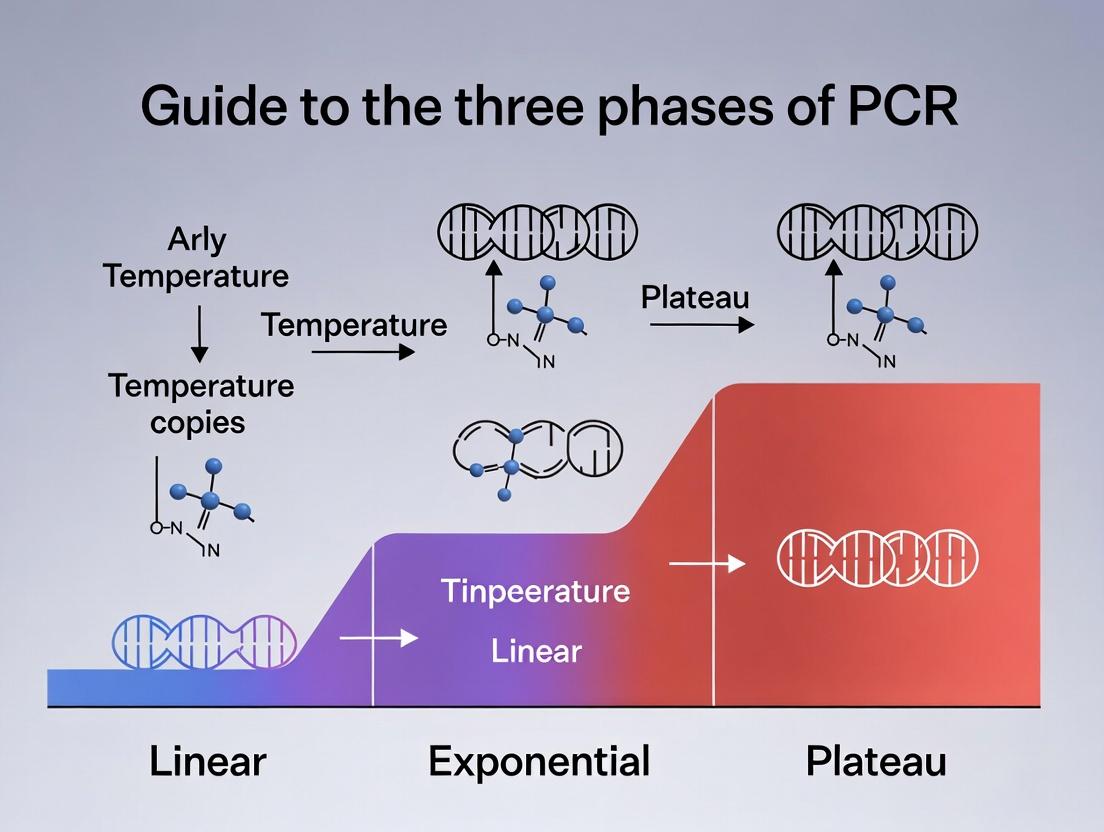
Within the framework of a comprehensive guide to the three phases of PCR—geometric, linear, and plateau—understanding the non-linear nature of the amplification curve is fundamental. The real-time PCR (qPCR) amplification plot, which tracks fluorescence versus cycle number, is sigmoidal, not linear. This shape is a direct consequence of the dynamic and changing efficiencies of the PCR reaction across its three kinetic phases.

The Three Kinetic Phases of PCR

The progression of a PCR reaction is not uniform. It can be delineated into three distinct phases, each governed by different limiting factors.

1. Geometric (Exponential) Phase: During early cycles, all reaction components are in excess. The amplification efficiency is at its maximum and constant, ideally doubling the target amplicon each cycle. The relationship is described by: [ Nn = N0 (1 + E)^n ] where (Nn) is the amplicon amount at cycle (n), (N0) is the initial amount, and (E) is the efficiency (0≤E≤1). In this phase, the log of the fluorescence increases linearly with cycle number. This is the only phase where quantitative analysis (quantification cycle, Cq) is valid.

2. Linear Phase: As the reaction progresses, one or more components (typically primers, dNTPs, or enzyme activity) become limiting. The efficiency begins to decrease with each subsequent cycle. Amplification continues, but the rate of increase slows progressively. The curve deviates from the straight line of the exponential log plot.

3. Plateau Phase: Reaction components are critically depleted, and product reannealing competes with primer binding. Net amplification efficiency approaches zero, and the fluorescence signal stabilizes, forming a plateau. The final yield is no longer correlated with the initial target amount.

The following table summarizes the defining characteristics of each PCR phase.

Table 1: Kinetic Parameters of the Three PCR Phases

Phase	Amplification Efficiency	Limiting Factors	Quantitative Utility
Geometric (Exponential)	Constant and maximal (ideally ~100%)	None; all components in excess	High; Cq value is used for reliable quantification
Linear	Declines progressively	Depletion of primers, dNTPs, enzyme activity	Low; not suitable for accurate quantification
Plateau	Near zero	Critical depletion of components, product reannealing	None; final yield is not template-dependent

Experimental Protocol: Monitoring PCR Kinetics via qPCR

This protocol outlines the generation of a standard amplification curve.

Objective: To generate and analyze a real-time PCR amplification curve, demonstrating the three kinetic phases. Method: SYBR Green I-based qPCR. Procedure:

• Reaction Setup: Prepare a master mix containing: 1X PCR buffer, 3.5 mM MgCl₂, 0.2 mM each dNTP, 0.5 µM each forward and reverse primer, 1X SYBR Green I dye, 1.25 units of hot-start DNA polymerase, and template DNA (e.g., a 10-fold serial dilution series). Adjust volume with nuclease-free water.
• Run qPCR: Load reactions into a real-time thermal cycler. Use a standard two-step protocol: Initial Denaturation: 95°C for 3 min; 40-45 cycles of: Denaturation: 95°C for 15 sec, Annealing/Extension: 60°C for 60 sec (with fluorescence acquisition at the end of this step).
• Data Analysis: The instrument software plots Raw Fluorescence (Rn) vs. Cycle Number. Apply baseline subtraction to correct for background fluorescence. The threshold line is set in the geometric phase of all reactions to determine the Cq value for each sample.
• Efficiency Calculation: From the dilution series, plot Cq values against the log of the starting template amount. The slope of the resulting standard curve is used to calculate efficiency: (E = 10^{-1/slope} - 1). An ideal reaction with 100% efficiency has a slope of -3.32.

Visualization of PCR Kinetics

The following diagram illustrates the relationship between cycle number, amplicon accumulation, and reaction efficiency.

Diagram 1: Dynamics of PCR phases, efficiency, and signal.

The Scientist's Toolkit: Key Research Reagent Solutions

Table 2: Essential Reagents for qPCR Kinetic Analysis

Reagent / Solution	Function & Importance in Kinetic Studies
Hot-Start DNA Polymerase	Minimizes non-specific amplification and primer-dimer formation during reaction setup, ensuring a cleaner, more efficient exponential phase crucial for accurate Cq determination.
SYBR Green I Dye	A double-stranded DNA intercalating dye that provides a fluorescent signal proportional to total amplicon mass, allowing real-time monitoring of product accumulation throughout all kinetic phases.
UltraPure dNTPs	High-purity deoxynucleotide triphosphates are essential for maintaining optimal and consistent reaction efficiency. Contaminants can alter kinetics and reduce yield.
Sequence-Specific Primers	Optimized primers with high purity and minimal self-complementarity are critical for achieving near-100% efficiency in the geometric phase and minimizing off-target products.
Nuclease-Free Water	The reaction solvent. Must be free of nucleases and PCR inhibitors to prevent enzyme degradation and skewed reaction kinetics.
Passive Reference Dye (ROX)	An inert fluorescence dye used in some systems to normalize for non-PCR-related fluctuations in well volume or signal intensity, improving data reproducibility.
Standard Template Dilution Series	A precise serial dilution of known template concentration is mandatory for constructing a standard curve to calculate PCR efficiency and validate kinetic performance.

Within the broader thesis on the Guide to the three phases of PCR geometric linear plateau research, this technical guide provides an in-depth analysis of the defining characteristics and underlying molecular events of the Exponential, Linear, and Plateau phases of the Polymerase Chain Reaction (PCR). Precise understanding of these phases is critical for optimizing assays in research, diagnostic, and drug development contexts.

The Three Phases of PCR

Exponential Phase (Geometric Phase)

This initial phase represents ideal amplification conditions where reaction components are in excess.

• Characteristics: The amount of PCR product doubles every cycle, following the theoretical equation N = N₀ × (1+E)^n, where E is amplification efficiency. The increase in product is best visualized on a log-linear plot.
• Molecular Events: All reagents (dNTPs, primers, Taq polymerase) are non-limiting. Primer annealing and extension are highly efficient. The DNA template is the single limiting factor. This is the only phase where quantitative data for qPCR (Cq values) is considered accurate.

Linear Phase

Amplification efficiency begins to decline as one or more reaction components become limiting.

• Characteristics: Product accumulation deviates from the ideal doubling curve, increasing in a near-linear fashion. The reaction rate slows progressively. Data from this phase is not reliable for quantification in qPCR.
• Molecular Events: Common limiting factors include the depletion of dNTPs or primers, inactivation of the DNA polymerase due to thermal cycling, competition from reannealing of complementary amplicon strands, and product inhibition. Enzyme-to-substrate ratios become suboptimal.

Plateau Phase

The reaction ceases to produce significant new amplicon molecules.

• Characteristics: The yield of amplified product stabilizes, forming the characteristic plateau in real-time amplification plots. The final yield is determined by the available reagents and experimental conditions.
• Molecular Events: Complete exhaustion of dNTPs or primers, full inactivation of polymerase, and significant competition from amplicon reannealing over primer annealing (leading to the formation of double-stranded product instead of new synthesis). Product inhibition (e.g., pyrophosphate buildup) may also contribute.

Table 1: Comparative Characteristics of PCR Phases

Phase	Amplification Efficiency	Product Accumulation	Key Limiting Factor	Quantitatively Reliable (qPCR)
Exponential	High & Constant (~100%)	Geometric (N = N₀ × 2^n)	Template DNA Concentration	Yes (Cq value)
Linear	Declining (from 100% to 0%)	Near-Linear	dNTPs, Primers, Enzyme Activity	No
Plateau	~0%	None	dNTPs, Primers, Enzyme, Amplicon Reannealing	No

Table 2: Typical Reaction Component Status by Phase

Component	Exponential Phase	Linear Phase	Plateau Phase
dNTPs	Vast Excess	Becoming Limiting	Exhausted
Primers	Vast Excess	Becoming Limiting	Exhausted
Taq Polymerase	Fully Active	Partial Inactivation	Fully Inactivated/Degraded
Template DNA	Limiting	No Longer Limiting	No Longer Limiting
Amplicon	Low Concentration	High Concentration	Very High Concentration

Experimental Protocols for Phase Analysis

Protocol 1: qPCR Standard Curve for Efficiency Determination

This protocol is used to determine the efficiency of the exponential phase.

• Sample Preparation: Prepare a serial dilution (e.g., 1:10) of a known template DNA over at least 5 orders of magnitude.
• qPCR Setup: Run each dilution in triplicate using a master mix containing SYBR Green dye or a sequence-specific probe.
• Cycling Conditions: Use standard cycling: Initial denaturation (95°C, 2-5 min); 40 cycles of [Denaturation (95°C, 10-30 sec), Annealing (Tm-specific, 15-30 sec), Extension (72°C, 15-30 sec/ kb)].
• Data Analysis: Plot the log of the initial template amount against the Cycle Quantification (Cq) value for each dilution. The slope of the linear regression is used to calculate efficiency: E = [10^(-1/slope)] - 1. An ideal efficiency of 100% (E=1.0) corresponds to a slope of -3.32.

Protocol 2: End-Point PCR for Plateau Yield Assessment

This protocol assesses factors affecting final yield in the plateau phase.

• Variable Testing: Set up identical PCR reactions, varying a single component (e.g., primer concentration from 0.1 µM to 1.0 µM, or dNTP concentration from 50 µM to 400 µM).
• PCR Amplification: Run for a high cycle number (e.g., 40 cycles) to ensure all reactions reach plateau.
• Product Quantification: Run PCR products on an agarose gel (e.g., 2%) alongside a DNA ladder. Stain with ethidium bromide or SYBR Safe. Quantify band intensity using gel documentation software.
• Analysis: Plot the concentration of the varied component against the final product yield (band intensity) to identify optimal concentrations and the point at which the component becomes non-limiting.

Visualizations

Diagram 1: PCR Phases Amplification Plot

Diagram 2: Molecular Events Driving Phase Transitions

The Scientist's Toolkit: Research Reagent Solutions

Table 3: Essential Reagents for PCR Phase Analysis

Reagent/Material	Function in Phase Analysis	Example/Note
Hot-Start DNA Polymerase	Reduces non-specific amplification during setup, ensuring a clean exponential phase baseline. Essential for high-sensitivity qPCR.	Immobilized antibodies or chemical modifications that inhibit activity until first denaturation.
SYBR Green I Dye	Intercalating dye for real-time monitoring of amplicon accumulation across all phases in qPCR.	Must use saturating dye concentrations; cheaper than probes but less specific.
Hydrolysis (TaqMan) Probes	Sequence-specific probes for highly specific detection during exponential phase, crucial for multiplex assays.	Provides superior specificity in complex biological samples for drug development research.
dNTP Mix	Building blocks for DNA synthesis. Concentration and purity directly impact linear and plateau phase yields.	Typical final concentration 200 µM each; unbalanced mixes lead to early plateau.
PCR Primers (Oligos)	Sequence-specific primers that define the amplicon. Concentration and design quality dictate exponential efficiency.	Optimized concentration typically 0.2-0.5 µM; design impacts primer-dimer formation.
qPCR Standard Template	Known concentration of template for generating standard curves to calculate exponential phase efficiency.	Often a plasmid or synthetic gBlock fragment; serial dilutions must be accurate.
Inhibitor-Removal Kits	Remove contaminants from samples (e.g., blood, soil) that can prematurely force reactions into linear phase.	Critical for reliable analysis from complex biological matrices in research.
ROX Passive Reference Dye	Normalizes for well-to-well variations in qPCR plate readers, ensuring accurate fluorescence measurement across phases.	Used in many real-time PCR instruments to correct for non-PCR related fluctuations.

In the canonical model of polymerase chain reaction (PCR) amplification, the process is described by three sequential phases: geometric (exponential), linear, and plateau. This whitepaper focuses exclusively on the geometric (exponential) phase, the foundational stage where amplification efficiency is theoretically optimal. The accurate identification and analysis of this phase is critical for precise nucleic acid quantification in research, clinical diagnostics, and drug development, particularly in qPCR and RT-qPCR assays. Understanding its theoretical underpinnings and critical assumptions is paramount for valid data interpretation across all applied fields.

Theoretical Foundations

The geometric phase is characterized by a perfect doubling of the target amplicon per cycle, assuming 100% amplification efficiency. The underlying kinetic model is described by the equation:

[ Nn = N0 \times (1 + E)^n ]

where:

• ( N_n ) = number of amplicon molecules after ( n ) cycles.
• ( N_0 ) = initial number of target molecules.
• ( E ) = amplification efficiency (ideally 1.0, or 100%).
• ( n ) = cycle number (within the geometric phase).

The relationship between fluorescence (ΔRn) and cycle number is exponential. The cycle threshold (Ct), a key quantitative output, is defined as the cycle number at which the fluorescence signal intersects a threshold line within this geometric phase.

Critical Assumptions of the Ideal Geometric Phase:

• Constant Maximum Efficiency: The amplification efficiency (E) is at its theoretical maximum and remains constant for all templates across all cycles within this phase.
• Unlimited Resource Availability: Reaction components (primers, nucleotides, polymerase) are in non-limiting excess and are equally accessible to all templates.
• Identical Template Integrity: All target molecules are intact and amplifiable with identical efficiency.
• No Inhibitory Agents: The reaction mixture is free of inhibitors that could reduce polymerase activity or primer annealing.
• Single-Predominant Product: Amplification yields a single, specific product without competitor artifacts (e.g., primer-dimers).

Deviations from these assumptions lead to non-ideal kinetics, premature transition to the linear phase, and quantification errors.

Table 1: Key Parameters Defining the Geometric Phase in qPCR

Parameter	Ideal Value	Typical Acceptable Range	Impact of Deviation
Amplification Efficiency (E)	1.00 (100%)	0.90 – 1.05 (90-105%)	Directly biases quantification of ( N_0 ); efficiency <90% reduces sensitivity.
Correlation Coefficient (R²) of Standard Curve	1.000	≥ 0.990	Indicates poor replicate consistency or variable efficiency across dilutions.
Replicate Variability (CV of Ct)	0%	< 1-2% for technical replicates	High CV indicates pipetting errors, template degradation, or inhibitor presence.
Dynamic Range	Not Applicable (Theoretical)	Typically 6-8 orders of magnitude	Narrow range suggests assay optimization failure or inhibition.

Table 2: Comparison of PCR Phases

Characteristic	Geometric (Exponential) Phase	Linear Phase	Plateau Phase
Primary Driver	Enzyme kinetics, template concentration.	Resource limitation (e.g., dNTPs, enzyme).	Product reannealing, enzyme inactivation, complete substrate consumption.
Efficiency (E)	Constant and maximal (~100%).	Declines progressively.	Approaches 0%.
Quantitative Utility	Essential for quantification (Ct value).	Not reliable for quantification.	No quantitative utility.
Signal-to-Noise Ratio	High.	Decreasing.	Variable, often high background.

Experimental Protocols for Validation

Validating that data is derived from a true geometric phase is a prerequisite for publication-quality work.

Protocol 4.1: Determining Amplification Efficiency via Standard Curve Objective: To calculate the actual amplification efficiency (E) of the assay and validate the linear dynamic range. Materials: See "Scientist's Toolkit" below. Procedure:

• Prepare a 10-fold serial dilution series (e.g., 10^6 to 10^1 copies/μL) of a known quantitated standard (e.g., gBlock, plasmid, cDNA).
• Amplify all dilutions in triplicate using the optimized qPCR assay.
• Record the Ct value for each replicate.
• Plot the mean log10(Starting Quantity) for each dilution against the mean Ct value.
• Perform linear regression. The slope of the line is used to calculate efficiency: ( E = 10^{-1/slope} - 1 ).
• Acceptance Criteria: Efficiency between 90-105% with R² ≥ 0.990.

Protocol 4.2: Assessing Reaction Kinetics with Fluorescence Derivative Analysis Objective: To visually identify the boundaries of the geometric phase and detect anomalies. Procedure:

• Following qPCR run, export the raw fluorescence data per cycle.
• Calculate the negative first derivative of the fluorescence curve (-d(RFU)/dCycle) to generate a peak-shaped profile.
• Plot the derivative versus cycle number. The geometric phase corresponds to the ascending slope and peak of the derivative curve.
• A single, sharp peak indicates a specific, efficient reaction. Multiple or broad peaks suggest non-specific amplification or inhibitor effects.

Visualization of Core Concepts

Title: Assumptions Underpinning Ideal Geometric Phase Data

Title: Transition Between PCR Phases

The Scientist's Toolkit: Essential Research Reagents & Materials

Table 3: Key Reagent Solutions for Geometric Phase Analysis

Reagent/Material	Function & Rationale	Critical for Validating Assumption
SYBR Green I Master Mix	Intercalating dye for dsDNA detection. Enables real-time monitoring of geometric phase kinetics.	Core assay component.
TaqMan Probe & Master Mix	Sequence-specific probe with fluorophore/quencher. Increases specificity, reducing non-geometric artifacts.	Assumption 5 (Single Product).
Nuclease-Free Water	Solvent and diluent. Prevents RNase/DNase degradation of templates and reagents.	Assumption 3 (Template Integrity).
Quantified Standard (gBlock, Plasmid)	Precisely known copy number for serial dilution. Essential for generating standard curve to calculate efficiency (E).	Validation of Assumption 1 (Constant E).
ROX Passive Reference Dye	Internal fluorescence normalization. Corrects for well-to-well volumetric variations, improving Ct precision.	Improves data quality for phase identification.
Inhibitor Removal Kit (e.g., SPRI beads)	Purification of sample nucleic acids. Removes contaminants (e.g., heparin, humic acid) that reduce efficiency.	Assumption 4 (No Inhibition).
High-Quality, Low-Edta TE Buffer	Resuspension buffer for primers and probes. Maintains stability without inhibiting polymerase (unlike EDTA).	Assumption 2 & 4 (Non-limiting, No Inhibition).
Digital Pipettes & Certified Low-Binding Tips	Ensure accurate, precise liquid handling for replicate reactions and serial dilutions.	Foundational for all quantitative assumptions.

Within the canonical three-phase model of Polymerase Chain Reaction (PCR) amplification—geometric (exponential), linear, and plateau—the linear phase represents a critical transition. This whitepaper provides an in-depth technical analysis of the linear phase, detailing the mechanistic causes for the departure from exponential growth, its quantitative characterization, and its implications for quantitative PCR (qPCR) assay design and data analysis for researchers and drug development professionals.

PCR amplification is not a perpetually exponential process. Efficiency, defined as the proportion of template molecules that are duplicated in each cycle, is not constant. The progression through three distinct phases is a fundamental concept for accurate nucleic acid quantification:

• Geometric/Exponential Phase: Ideal conditions with maximal reaction efficiency (~100%). Template concentration is below inhibitory levels, and reagents are in excess.
• Linear Phase: Reaction efficiency begins to decline perceptibly. Amplification is no longer exponential but follows a near-linear trajectory on a semi-log plot.
• Plateau Phase: Reaction efficiency approaches zero. Amplification ceases due to depletion of reagents or inhibition by reaction products.

This document focuses on the Linear Phase as the transition zone, examining the factors that cause efficiency loss and how to model and utilize this phase in experimental workflows.

Quantitative Characterization of the Linear Phase

The linear phase is quantitatively defined by a cycle-dependent decrease in amplification efficiency (E). During the exponential phase, E is constant (E ≈ 1). The onset of the linear phase is marked by E < 1, decreasing with each subsequent cycle until E ≈ 0 at the plateau.

Table 1: Key Quantitative Parameters Across PCR Phases

Phase	Amplification Efficiency (E)	Reaction Rate Constant (k)*	[dNTPs] / [Primers] Status	[Amplicon] Relative to Inhibitor Threshold
Geometric/Exponential	~1.0 (100%)	High, constant	Large excess (>10:1)	Well below
Linear	1.0 > E > 0.1	Decreasing cycle-by-cycle	Becoming limiting (<5:1)	Approaching
Plateau	~0.0 (0%)	~0	Critically limiting or depleted	Far above

*The apparent first-order rate constant for product formation.

Table 2: Primary Causes of Linear Phase Onset and Their Experimental Signatures

Cause	Underlying Mechanism	Observable Experimental Signature in qPCR
dNTP Depletion	Substrate concentration falls below Km of DNA polymerase.	Reduced yield per cycle; can be delayed by increasing initial [dNTP].
Primer Depletion	Primer:template ratio drops, slowing annealing kinetics.	Asymmetric amplification; primer-dimers may become prevalent.
Polymerase Inactivation	Thermal denaturation or product inhibition reduces active enzyme.	Progressive slowdown insensitive to reagent re-spiking.
Pyrophosphate Inhibition	Accumulation of PPi chelates Mg2+, a required cofactor.	Can be mitigated by inclusion of pyrophosphatase.
Competition for Reagents	Non-specific products (e.g., primer-dimers) consume dNTPs/primer.	High background fluorescence, abnormal melt curves.
Amplicon Re-annealing	At high [dsDNA], complementary strands re-anneal faster than primer binding.	Strongly dependent on amplicon length and GC content.

Core Experimental Protocol: Quantifying Amplification Efficiency

To empirically determine the efficiency curve and identify the linear phase onset, a standard curve protocol is essential.

Protocol: Standard Curve for Efficiency Analysis

• Template Preparation: Serially dilute (typically 10-fold) a known quantity of target template (e.g., gDNA, plasmid) over at least 5 orders of magnitude.
• qPCR Setup: Run all dilutions in triplicate using the same master mix and cycling conditions.
• Data Analysis:
  • Plot Cq (Quantification Cycle) values vs. log10(Starting Quantity).
  • Perform linear regression. The slope is used to calculate efficiency: E = 10^(-1/slope) - 1.
  • Ideal (Exponential Phase): Slope ≈ -3.32, E ≈ 1.0.
  • Linear Phase Onset: Deviations from linearity at high template concentrations indicate early efficiency loss. The point where the measured Cq consistently deviates above the regression line marks the start of the linear phase for that assay.

Signaling Pathways and Reaction Dynamics

The shift from exponential to linear growth is governed by the dynamic interplay of reaction components. The core pathway of PCR amplification and its points of inhibition are visualized below.

Diagram Title: PCR Cycle with Linear Phase Inhibition Points

The Scientist's Toolkit: Essential Research Reagent Solutions

Table 3: Key Reagents for Studying and Controlling the Linear Phase

Item	Function in Context of Linear Phase	Example/Note
Hot-Start DNA Polymerase	Reduces non-specific amplification and primer-dimer formation, delaying reagent competition and extending exponential phase.	Chemically modified or antibody-bound enzymes.
dNTP Mix, High Concentration	Increases substrate reservoir, directly delaying depletion-caused linear phase onset.	Use 200-500 µM each dNTP final concentration.
MgCl₂ Optimization Buffer	Mg2+ is a critical cofactor; its optimal concentration stabilizes enzymes and primers, maximizing efficiency.	Often requires titration (1.5-5.0 mM).
PCR Additives (e.g., BSA, DMSO)	Reduces enzyme inhibition by sample contaminants and mitigates secondary structure, improving efficiency.	Helpful for complex templates (e.g., GC-rich).
Passive Reference Dye (ROX)	Normalizes for well-to-well volume variations in qPCR, critical for accurate fluorescence measurement in late cycles.	Essential for multi-well plate instruments.
SYBR Green I Dye	Intercalating dye for monitoring dsDNA accumulation. Signal saturation in late cycles is a hallmark of plateau.	Use at optimal, non-inhibitory concentration.
Uracil-DNA Glycosylase (UDG)	Prevents carryover contamination, ensuring early cycle exponential growth is not skewed by background.	Used with dUTP-incorporated dNTP mixes.
Digital PCR Partitioning Oil/Reagent	For absolute quantification, partitions sample to achieve <1 template/partition, ensuring exponential amplification in each.	Eliminates the need for standard curves.

Advanced Analysis: Modeling the Linear Phase

The transition can be modeled mathematically. A commonly adapted model is the saturation growth model: [ Fn = \frac{F{max}}{1 + e^{-k(n - n{1/2})}} ] Where (Fn) is fluorescence at cycle (n), (F{max}) is maximum fluorescence, (k) is the rate constant, and (n{1/2}) is the inflection point cycle. The derivative of this curve ((dF/dn)) shows efficiency dropping from a constant maximum to zero. The linear phase occupies the region around the inflection point where the second derivative is near zero.

Experimental Workflow for Model Validation:

Diagram Title: Workflow for qPCR Linear Phase Analysis

Implications for Drug Development and Research

• qPCR Assay Validation: The linear phase defines the Upper Limit of Quantification (ULOQ). Samples with Cq values within the linear phase require dilution for accurate quantification.
• Diagnostic Assay Design: For binary (yes/no) outcomes, assay conditions can be optimized to ensure target-positive samples clearly exit the linear phase within a defined cycle threshold.
• Gene Expression Analysis (ΔΔCq): Critical Requirement: All samples and controls must be compared within the exponential phase. Using data from the linear phase introduces significant error due to variable efficiency.
• Inhibitor Screening: The sensitivity of the linear phase onset to inhibitors makes it a potential marker for screening compound libraries for molecules that affect nucleic acid metabolism.

The linear phase is not an artifact but an inevitable thermodynamic and kinetic consequence of finite reaction components and accumulating products. A precise understanding of its causes—depletion, inhibition, and competition—enables robust experimental design, accurate data interpretation, and reliable diagnostic and drug development outcomes. By optimizing reagent solutions and rigorously defining the exponential-linear transition, researchers can ensure their quantitative results are derived from the phase of maximum and constant efficiency.

Within the canonical framework of PCR kinetics—Geometric, Linear, and Plateau phases—the final plateau phase represents a critical inflection point where reaction efficiency drops to zero. This in-depth technical guide examines the plateau phase not as a mere endpoint, but as a complex, limitation-driven state. Understanding its underlying causes is paramount for accurate quantitative analysis, assay optimization, and reliable interpretation in research and diagnostic applications, forming a cornerstone of a comprehensive thesis on the "Guide to the three phases of PCR (geometric, linear, plateau) research."

Core Mechanisms Leading to the Plateau

The cessation of exponential product accumulation is multifactorial, primarily driven by substrate depletion and enzyme inactivation.

2.1. Key Limiting Factors

• dNTP and Primer Depletion: As the concentration of amplicon exceeds that of the initial dNTPs or primers, these substrates become exhausted, halting chain elongation.
• Taq DNA Polymerase Inactivation: Despite being thermostable, the polymerase undergoes gradual thermal denaturation over many cycles, reducing available active enzyme.
• Product Reassociation (Competitive Inhibition): The high concentration of double-stranded PCR product (amplicon) outcompetes primers for binding to the template. Reannealing of complementary amplicon strands prevents primer binding and extension.
• Inhibition by Pyrophosphate: Accumulation of pyrophosphate (a byproduct of dNTP incorporation) can form insoluble complexes with magnesium, a critical cofactor for polymerase activity.
• Incomplete Strand Separation: At later cycles, high product concentrations can lead to incomplete denaturation, reducing available single-stranded template.

Table 1: Quantitative Impact of Common Limiting Factors in Late-Cycle PCR

Limiting Factor	Typical Initial Concentration	Estimated Concentration at Plateau (for a robust 30μL reaction)	Primary Consequence
dNTPs	200 μM each	< 10 μM	Cessation of primer extension
Primers	0.2 - 1.0 μM each	< 0.01 μM	No new initiation events
Active Taq Polymerase	1.25 Units	< 0.25 Units	Drastic reduction in synthesis rate
Mg²⁺ (free)	1.5 mM	Variable, significantly reduced	Reduced polymerase fidelity & rate
Amplicon Concentration	0	~10⁻⁹ M (nM range)	Competitive inhibition & reannealing

Experimental Protocol: Quantifying Plateau Phase Dynamics

This protocol outlines a method to systematically investigate factors influencing the plateau phase.

Title: Monitoring PCR Efficiency Decline via Serial Dilution and Extended Cycling.

Objective: To correlate initial template concentration with the cycle number at which the reaction enters the plateau phase, and to assess product yield after excessive cycling.

Materials (Research Reagent Solutions):

• Master Mix: High-fidelity or standard Taq DNA polymerase mix, containing buffer, MgCl₂, and dNTPs.
• Target Primers: Validated, lyophilized primers resuspended in nuclease-free water to a 100 μM stock.
• Template DNA: Quantified genomic DNA or plasmid containing the target sequence.
• Intercalating Dye: SYBR Green I, at the manufacturer's recommended dilution.
• qPCR Instrument: Calibrated real-time PCR system.

Methodology:

• Prepare a 10-fold serial dilution of the template DNA across at least 6 orders of magnitude (e.g., from 10 ng/μL to 0.001 pg/μL).
• For each dilution, prepare replicate reactions containing 1X Master Mix, 0.3 μM each primer, 1X SYBR Green I, and 5 μL of template.
• Run the qPCR with an extended cycle protocol:
  • Initial Denaturation: 95°C for 3 min.
  • 50-60 Cycles of:
    • Denaturation: 95°C for 15 sec.
    • Annealing: 60°C for 20 sec.
    • Extension: 72°C for 30 sec.
  • Plate read at the end of each extension step.
• After the final cycle, perform a melt curve analysis from 65°C to 95°C to confirm product specificity.

Data Analysis:

• Plot fluorescence (Rn) vs. cycle number for all dilutions.
• Record the Cycle Threshold (Ct) for each sample.
• For each reaction, identify the cycle at which the fluorescence curve visibly deviates from exponential growth and flattens (Plateau Onset Cycle).
• Record the Final Fluorescence Plateau Height for each reaction.
• Analyze the relationship between initial template amount, Ct, Plateau Onset Cycle, and Plateau Height.

Visualization of PCR Phase Kinetics and Limitations

Diagram Title: PCR Phase Transitions and Limiting Factors

Diagram Title: Amplicon-Driven Inhibition at Plateau

The Scientist's Toolkit: Essential Reagents for Plateau Phase Studies

Table 2: Key Research Reagent Solutions for PCR Limitation Analysis

Reagent / Material	Primary Function in Plateau Phase Research
Hot-Start Taq DNA Polymerase	Reduces non-specific amplification and primer-dimer formation early on, ensuring more reagent is available for later cycles, potentially delaying plateau.
dNTP Mix (25 mM each)	Standard substrate for elongation. Systematic variation of its concentration (e.g., from 50 μM to 400 μM) directly tests substrate limitation hypotheses.
MgCl₂ Solution (25 mM)	Critical cofactor for polymerase activity. Titration is essential as its free concentration is affected by dNTP and amplicon concentration.
SYBR Green I Dye	Intercalating dye for real-time fluorescence monitoring of product accumulation. Allows precise determination of the cycle where fluorescence growth deviates from exponential.
Passive Reference Dye (ROX)	Normalizes for well-to-well variations in reaction volume or fluorescence, critical for accurate plateau height comparison across samples.
qPCR Plates with Optical Seals	Ensure consistent thermal conductivity and prevent evaporation during extended cycling (e.g., 60+ cycles) required to fully observe the plateau.
Nuclease-Free Water	Critical for diluting stocks and setting up reactions; prevents enzymatic degradation of primers, templates, and reagents.

Within the broader thesis of A Guide to the Three Phases of PCR: Geometric, Linear, Plateau, understanding the core quantitative parameters of real-time quantitative PCR (qPCR) is fundamental. These parameters are the linchpins for accurate data interpretation across all amplification phases. This technical guide provides an in-depth analysis of Cycle Threshold (C_T/C_q) values, amplification efficiency, and baseline fluorescence, detailing their calculation, optimization, and impact on quantitative analysis.

CT/CqValue: The Primary Quantitative Metric

The Cycle Threshold (C_T) or Quantification Cycle (C_q) is the cycle number at which the amplification fluorescence signal crosses a defined threshold above the baseline. It is the primary output for quantification, inversely proportional to the log of the initial target amount.

Calculation and Determination: The threshold is typically set within the exponential (geometric) phase of amplification, 3-5 standard deviations above the mean baseline fluorescence. Most software algorithms automatically set the threshold, but manual verification is critical.

Amplification Efficiency: The Foundation of Accurate Quantification

Amplification efficiency (E) describes the rate of product doubling per cycle during the exponential phase. An ideal reaction has an efficiency of 100% (E=2.0), meaning the product doubles every cycle.

Determination via Standard Curve: Efficiency is derived from the slope of a standard curve generated from serial dilutions of a known template: [ E = 10^{(-1/slope)} - 1 ] or as a percentage: [ \%E = (E \times 100)\% ].

Table 1: Interpretation of Amplification Efficiency

Slope	Efficiency (E)	Percentage (%)	Interpretation
-3.322	2.00	100%	Ideal doubling
-3.58	1.90	90%	Acceptable range
-3.10	2.11	111%	May indicate inhibition or artifact
< -3.9 or > -3.0	< 1.80 or > 2.20	<80% or >120%	Requires investigation

Baseline Fluorescence: Defining the Signal Background

The baseline is the initial PCR cycles where fluorescence signal accumulates below the detection threshold, primarily from background signals and unincorporated probes/dyes. Correct baseline setting is crucial for accurate C_q determination.

Establishment Protocol: The baseline is typically set from cycles 3-15, but this should be adjusted to end just before the earliest amplification signal is observed. The baseline fluorescence is subtracted from all raw fluorescence data.

Table 2: Common Sources of Baseline Fluorescence

Source	Contribution	Mitigation Strategy
Unincorporated SYBR Green dye	High	Optimize dye concentration; use passive reference dyes.
Probe fluorescence (Hydrolysis probes)	Low-Medium	Ensure proper probe design and quenching.
Tube/plate fluorescence	Variable	Use optically clear, low-fluorescence plastics.
Instrument noise	Variable	Regular calibration and maintenance.

Experimental Protocols

Protocol 1: Determining Amplification Efficiency via Standard Curve

• Template Preparation: Prepare a 5- or 10-fold serial dilution series (e.g., 1:10, 1:100, 1:1000) of a known template (cDNA, gDNA, plasmid). Use at least 5 dilution points.
• qPCR Setup: Run all dilutions in triplicate on the same plate with your target assay (primers/probe).
• Data Analysis: Plot the mean C_q value for each dilution against the log₁₀ of its starting quantity/concentration.
• Linear Regression: Perform a linear fit. The slope and R² are reported.
• Calculate Efficiency: Apply the formula ( E = 10^{(-1/slope)} ). Assess using Table 1.

Protocol 2: Validating Baseline and Threshold Settings

• Run No-Template Controls (NTCs): Include multiple NTCs to assess background.
• Visual Inspection: Examine the amplification plot. The baseline should encompass cycles where all amplification curves (including NTCs) are flat and parallel.
• Manual Adjustment: If automatic baseline is incorrect, manually set the baseline end cycle to 1-2 cycles before the earliest true amplification signal rises. Set the threshold within the exponential phase of all target amplifications, well above any NTC signal.

Visualizing qPCR Parameter Relationships

Diagram 1: Relationship of core qPCR parameters in quantification.

The Scientist's Toolkit: Essential Research Reagent Solutions

Table 3: Key Reagents for Robust qPCR Parameter Analysis

Reagent/Material	Function & Importance
High-Fidelity DNA Polymerase Mix	Provides robust, efficient amplification with high fidelity, critical for accurate standard curve generation.
dNTP Mix (balanced)	Ensures equal incorporation rates; imbalances can reduce amplification efficiency.
Optical-Grade Plate Seals	Prevents well-to-well contamination and evaporation, ensuring stable baseline fluorescence.
Passive Reference Dye (e.g., ROX)	Normalizes for non-PCR related fluorescence fluctuations between wells, stabilizing baseline.
Commercial qPCR Master Mix	Pre-optimized buffer, enzyme, dNTPs, and dye for consistent efficiency and baseline performance.
Nuclease-Free Water	Prevents degradation of primers, probes, and templates, a critical control for NTCs.
Synthetic Oligonucleotide Standards (gBlocks)	Provides absolute, sequence-specific standards for highly precise efficiency calculations.
Inhibitor Removal Kit (e.g., for blood, soil)	Removes PCR inhibitors present in biological samples that drastically reduce efficiency.

Mastering C_T/C_q values, amplification efficiency, and baseline fluorescence is not an isolated task but a continuous requirement for valid interpretation across the geometric, linear, and plateau phases of PCR. Proper experimental design, rigorous protocol execution, and vigilant data analysis of these parameters form the bedrock of reliable, reproducible qPCR data essential for research and drug development.

The analysis of the Polymerase Chain Reaction (PCR) through its geometric, linear, and plateau phases is fundamental to quantitative molecular biology. This evolution, from empirical observation to a cornerstone of quantitative PCR (qPCR), reflects the integration of thermodynamics, enzyme kinetics, and sophisticated detection systems. This guide situates this technical evolution within the broader thesis of a "Guide to the three phases of PCR geometric linear plateau research," providing the experimental and theoretical framework for modern application.

1. The Three Phases: Theoretical Foundation and Historical Recognition

The characteristic sigmoidal curve of product accumulation was first empirically described in the early publications on PCR. The formalization into distinct phases provided the critical insight that only the exponential (geometric) phase is a true indicator of initial target quantity.

• Geometric/Exponential Phase: Ideal doubling per cycle occurs. Efficiency is maximal and constant. This phase is the only reliable region for quantitative analysis.
• Linear Phase: Reaction efficiency declines due to reagent depletion (dNTPs, primers), enzyme inactivation, and product reannealing competing with primer binding. Quantification is inaccurate in this phase.
• Plateau Phase: Reaction has ceased; product accumulation is negligible. Endpoint analysis, used in early PCR, is highly variable and non-quantitative.

The shift from endpoint to kinetic analysis, enabled by the advent of real-time fluorescence detection, was the pivotal moment that transformed phase analysis from a descriptive concept into a precise quantitative tool.

Table 1: Evolution of PCR Analysis Paradigms

Era	Analysis Type	Primary Phase Utilized	Key Limitation	Quantitative Capability
Pre-1990s	Endpoint	Plateau	High variability, post-amplification handling	Qualitative/Semi-quantitative
1990s	Kinetic (Real-time)	Geometric/Exponential	Relies on robust early-cycle fluorescence detection	Highly Quantitative (Absolute & Relative)
2000s-Present	Digital (dPCR)	Endpoint (Binary)	Throughput and dynamic range constraints	Absolute Quantification without standard curves

2. Experimental Protocol: qPCR Efficiency Determination (Linear Regression)

This protocol is essential for validating that an assay operates in the ideal geometric phase across a dilution series.

Objective: To calculate the amplification efficiency (E) of a qPCR assay by constructing a standard curve from serially diluted template. Materials:

• Template DNA: Known concentration (e.g., genomic DNA, plasmid, PCR product).
• qPCR Master Mix: Contains hot-start DNA polymerase, dNTPs, MgCl2 in optimized buffer.
• Primer Pair: Target-specific, optimally designed (amplicon 70-200 bp).
• Fluorophore: SYBR Green I dye or target-specific hydrolysis (TaqMan) probe.
• qPCR Instrument: Thermocycler with real-time fluorescence detection capability.

Procedure:

• Prepare Dilution Series: Create a 10-fold serial dilution of the template (e.g., across 6 orders of magnitude). Use nuclease-free water or TE buffer.
• Plate Setup: In triplicate, load reactions for each dilution. Include a no-template control (NTC).
• Reaction Assembly (20µL typical):
  • 10µL 2x qPCR Master Mix
  • Forward & Reverse Primer (final concentration 200-500 nM each)
  • Fluorophore (if not pre-included in master mix)
  • Template DNA (variable volume)
  • Nuclease-free water to 20µL
• Run qPCR Program:
  • Initial Denaturation: 95°C for 2-5 min.
  • 40-45 Cycles of:
    • Denaturation: 95°C for 10-30 sec.
    • Annealing/Extension: 60°C for 30-60 sec (acquire fluorescence).
• Data Analysis:
  • Determine the quantification cycle (Cq) for each replicate.
  • Plot the mean log10(Starting Quantity) for each dilution against its mean Cq value.
  • Perform linear regression. The slope of the line is used to calculate efficiency: Efficiency (E) = [10^(-1/slope) - 1] * 100%.
  • An ideal reaction (100% efficient, perfect doubling) has a slope of -3.32 and E=100%. Acceptable range is 90-110% (slope between -3.58 and -3.10).

Table 2: Interpretation of qPCR Efficiency Metrics

Slope	Efficiency (E)	Interpretation	Action
-3.10 to -3.58	90% - 110%	Optimal. Assay is suitable for precise quantification.	Proceed.
> -3.10	> 110%	Inhibition or poor assay optimization. Reaction is super-optimal.	Re-optimize primer concentrations, Mg2+ levels, or template purity.
< -3.58	< 90%	Inhibition, poor primer design, or sub-optimal conditions.	Check for inhibitors, re-design primers, optimize annealing temperature.

3. Diagram: The Three Phases of PCR and Analysis Methods

The Scientist's Toolkit: Key Research Reagent Solutions

Table 3: Essential Reagents for PCR Phase Analysis

Reagent/Material	Function in Phase Analysis	Critical Consideration
Hot-Start DNA Polymerase	Prevents non-specific amplification during reaction setup, ensuring a clean baseline and accurate early-cycle (geometric phase) fluorescence detection.	Essential for robust Cq values and high amplification efficiency.
qPCR Master Mix (Optimized Buffer)	Provides optimal pH, salt, and MgCl2 concentration. Stabilizes enzyme, maximizes efficiency, and ensures consistent progression through phases.	Includes dNTPs; Mg2+ concentration is a key optimization variable.
Fluorogenic Probe (TaqMan)	Target-specific hydrolysis probe provides sequence confirmation, enabling multiplexing. Signal is directly proportional to amplicon yield.	More specific than intercalating dyes; requires separate probe design.
Intercalating Dye (SYBR Green I)	Binds double-stranded DNA, providing universal detection. Monitors total product accumulation through all phases.	Requires melt curve analysis post-run to verify amplicon specificity.
Nuclease-Free Water	Solvent for all reactions; ensures no contaminating RNases, DNases, or inhibitors that could alter reaction efficiency and phase kinetics.	Critical for reproducibility and avoiding false negatives in low-template reactions.
Standard Reference Material	Known concentration template for constructing standard curves. Allows conversion of Cq to target quantity and calculation of efficiency.	Must be of high purity and accurately quantified; matrix-matched to samples if possible.

Practical Applications: How to Leverage PCR Phases for Accurate Quantification and Assay Design

Quantitative PCR (qPCR) remains the gold standard for nucleic acid quantification. Its amplification profile is universally described by three phases: geometric (or exponential), linear, and plateau. Reliable and precise quantification depends exclusively on data from the geometric phase, where reaction efficiency is constant and maximal. This guide, framed within a broader thesis on the Guide to the three phases of PCR (geometric, linear, plateau) research, details how to design experiments that explicitly target the geometric phase for robust results in research and drug development.

The Criticality of the Geometric Phase

During the geometric phase, the amount of PCR product ideally doubles each cycle (100% efficiency). This predictability allows for accurate calculation of initial template concentration. The linear phase sees declining efficiency due to reagent depletion, and the plateau phase is characterized by reaction cessation, both rendering data from these phases quantitatively unreliable.

Table 1: Characteristics of qPCR Amplification Phases

Phase	Reaction Efficiency	Key Influencing Factors	Suitability for Quantification
Geometric (Exponential)	Constant & High (~100%)	Primer design, template quality, master mix composition	Ideal: Direct relationship between Cq and log(initial template)
Linear	Declining ( < 100%)	Depletion of dNTPs, primers, enzyme activity	Unreliable: Variable efficiency prevents accurate quantification
Plateau	Near 0%	Exhaustion of reagents, product re-annealing, inhibition	Unusable: No correlation with initial template amount

Core Principles for Geometric Phase-Targeted Design

Defining the Quantification Cycle (Cq)

The Cq (Quantification Cycle) is the pivotal data point, representing the cycle at which the amplification curve crosses the threshold line. It must be derived from the geometric phase.

• Threshold Setting: Set within the geometric phase's linear region on the log(fluorescence) vs. cycle plot, typically 10 standard deviations above the baseline fluorescence.

Optimizing Reaction Efficiency

To ensure the Cq lies within the true geometric phase, reaction efficiency (E) must be optimized and validated.

• Efficiency Calculation: Derived from the slope of a standard curve: E = 10^(-1/slope) - 1. Ideal efficiency is 100% (slope = -3.32).
• Acceptable Range: 90-110% (slope between -3.58 and -3.10).

Table 2: Impact of Reaction Efficiency on Quantification Accuracy

Efficiency	Slope (of std curve)	Fold Change Error per Cycle*	Impact on Relative Quantification (ΔΔCq)
100%	-3.32	0%	Accurate
110%	-3.10	+4.5%	Underestimation of fold-change
90%	-3.58	-5.3%	Overestimation of fold-change
80%	-3.81	-11%	Severe bias

Example: For a 5 Cq difference, 90% efficiency introduces a ~1.3-fold error.

Assay Validation Protocol

• Standard Curve Dilution Series: Prepare a 5-10 point serial dilution (e.g., 1:5 or 1:10) of known template. Run in triplicate.
• Analysis: Plot log(initial quantity) vs. Cq. Calculate slope, R², and efficiency. R² should be >0.99.
• Dynamic Range: The geometric phase is maintained across all dilutions used for quantification.

Experimental Protocol: A Geometric Phase-Focused qPCR Workflow

Objective: To quantify gene expression in treated vs. control samples with data derived strictly from the geometric phase.

Step 1: Assay Design & Validation

• Design primers with stringent criteria: amplicon length 80-150 bp, Tm 58-60°C, minimal secondary structure.
• Clone target amplicon into a plasmid. Prepare a 6-point 1:10 serial dilution (e.g., from 10^6 to 10^1 copies/µL).
• Run qPCR with this standard curve alongside a no-template control (NTC).
• Validation Criteria: Efficiency = 90-110%, R² > 0.99. The NTC must show no amplification or a Cq > 40.

Step 2: Sample Preparation & Reverse Transcription

• Extract total RNA using a silica-column method. Measure concentration and purity (A260/A280 ~2.0).
• Treat with DNase I to remove genomic DNA.
• Perform reverse transcription for all samples using a fixed amount of RNA (e.g., 1 µg) with anchored oligo(dT) or random hexamer primers. Include a no-reverse transcriptase (-RT) control for each sample.

Step 3: qPCR Setup for Target & Reference Genes

• Prepare a master mix containing: 10 µL 2x SYBR Green Master Mix, 0.8 µL forward primer (10 µM), 0.8 µL reverse primer (10 µM), 6.4 µL nuclease-free water, and 2 µL cDNA template (diluted 1:10).
• Load samples in triplicate (biological and technical) for both target genes and stable reference genes (e.g., GAPDH, ACTB).
• Run on qPCR instrument with cycling: Initial denaturation (95°C, 2 min); 40 cycles of [95°C for 15 sec, 60°C for 1 min (acquire fluorescence)].

Step 4: Data Analysis Targeting Geometric Phase

• Set the fluorescence threshold in the instrument's software within the linear region of the geometric phase for all plates.
• Export Cq values. Calculate relative quantification using the ΔΔCq method, which is valid only when efficiencies of target and reference genes are approximately equal and near 100%.
  • ΔCq (sample) = Cq(target) - Cq(reference)
  • ΔΔCq = ΔCq(treated) - ΔCq(control)
  • Fold Change = 2^(-ΔΔCq)

Visualization: qPCR Experimental Workflow & Phase Logic

Geometric Phase qPCR Workflow

qPCR Phases & Quantification Suitability

The Scientist's Toolkit: Essential Research Reagent Solutions

Table 3: Key Reagents for Robust Geometric Phase qPCR

Reagent / Material	Function in Targeting Geometric Phase	Key Considerations
Hot-Start DNA Polymerase	Reduces non-specific amplification and primer-dimer formation during setup, preserving reagents for the true geometric phase.	Enzymes with antibody or chemical modification offer stringent hot-start.
SYBR Green or Hydrolysis Probe Master Mix	Contains optimized buffer, dNTPs, and polymerase for consistent, high-efficiency amplification. Use a master mix for reproducibility.	Choose mixes with inhibitors of genomic DNA amplification if needed.
Ultra-Pure dNTPs	Balanced, high-purity nucleotides are essential substrates for maintaining 100% efficiency during geometric phase.	Degraded dNTPs reduce efficiency and shorten geometric phase.
Validated Primer Pairs	Specific primers with high on-target efficiency are the foundation for a long, stable geometric phase.	Must be validated with a standard curve. Avoid secondary structure.
Nuclease-Free Water	Prevents degradation of primers, templates, and enzymes, which would shorten the geometric phase.	A critical, often overlooked component for assay robustness.
Standard Curve Template (e.g., gBlock, Plasmid)	Provides known-copy-number standards to calculate reaction efficiency and validate the geometric phase range.	Essential for absolute quantification and for validating any assay.
ROX Passive Reference Dye	Normalizes for well-to-well fluorescence fluctuations, ensuring accurate threshold calling in the geometric phase.	Required for some instruments; check manufacturer guidelines.

Accurate qPCR quantification is not merely a function of measuring fluorescence; it is a deliberate exercise in confining data analysis to the geometric amplification phase. By rigorously validating assays, optimizing reagents, and setting analytical parameters within this window of constant efficiency, researchers can generate reliable, reproducible data. This targeted approach, central to a comprehensive understanding of PCR kinetics, is indispensable for meaningful conclusions in basic research and critical decision-making in drug development.

This guide is framed within the broader thesis of "A Guide to the Three Phases of PCR: Geometric, Linear, and Plateau," which provides a foundational framework for understanding qPCR kinetics. Accurate quantification in quantitative PCR (qPCR) is contingent upon a precise understanding of these distinct amplification phases. The choice between absolute and relative quantification is not arbitrary; it is a strategic decision heavily influenced by which phase of the PCR curve is being analyzed and the specific experimental question. This whitepaper delves into the technical considerations for selecting the appropriate quantification method based on phase characteristics, ensuring data integrity for researchers, scientists, and drug development professionals.

The Three Phases of PCR and Quantification Relevance

• Geometric (Exponential) Phase: Ideal for quantification. In this phase, the amplification efficiency is at its maximum and constant. The amount of PCR product doubles with each cycle, and the cycle threshold (Cq) is directly proportional to the initial amount of target. Both absolute and relative quantification methods rely on data from this phase.
• Linear Phase: Amplification efficiency begins to decline due to limiting reagents (e.g., enzymes, nucleotides). Quantification based on endpoint measurements in this phase is highly unreliable and should be avoided for primary analysis.
• Plateau Phase: Reaction components are exhausted, and product accumulation ceases. Fluorescence signal plateaus. No meaningful quantitative data can be derived from this phase.

Core Quantification Methods: Principles and Phase Dependence

Absolute Quantification

This method determines the exact copy number or concentration of a target sequence in a sample by comparing its Cq value to a standard curve of known concentrations.

• Phase Dependence: Exclusively utilizes the Cq value, which is a derivative of the geometric phase. The standard curve must be run under identical conditions (same efficiency) as the samples.
• Primary Use: Viral load testing, pathogen quantification, copy number variation analysis, and gene expression where absolute transcript numbers are required.

Relative Quantification

This method determines the fold-change in target nucleic acid quantity relative to a calibrator sample (e.g., untreated control) and one or more reference genes. It does not require a standard curve of the target.

• Common Models:
  • ΔΔCq (Livak) Method: Assumes the amplification efficiencies of the target and reference genes are approximately equal and close to 100%.
  • Pfaffl Model: Incorporates actual, calculated amplification efficiencies for both target and reference genes, offering greater accuracy when efficiencies are not equal.
• Phase Dependence: Relies on the comparison of Cq values (from the geometric phase) between targets and reference genes. Accurate efficiency determination is critical.

Table 1: Comparison of Absolute and Relative Quantification

Feature	Absolute Quantification	Relative Quantification (ΔΔCq)	Relative Quantification (Pfaffl)
Output	Exact copy number or concentration	Fold-change relative to a calibrator	Fold-change relative to a calibrator
Requires Standard Curve	Yes, for target gene	No (but requires reference gene curve)	No (but requires reference gene curve)
Key Phase Used	Geometric (Cq value)	Geometric (Cq value)	Geometric (Cq value & efficiency)
Efficiency Consideration	Critical; standard curve defines run efficiency	Assumes target and ref. efficiency = 100%	Incorporates actual calculated efficiencies
Primary Application	Viral loads, copy number, absolute transcript count	Gene expression profiling, pathway analysis	Gene expression when efficiencies differ
Throughput	Lower (requires full standard curve)	High	High
Major Assumption	Sample and standard amplify with identical efficiency	Target and reference genes amplify with equal and perfect efficiency	Amplification kinetics are modeled accurately

Table 2: Suitability of Quantification Method Based on Experimental Phase & Goal

Experimental Goal / Phase Characteristic	Recommended Method	Rationale
Determining absolute pathogen copy number	Absolute Quantification	Only method that provides a concrete concentration value.
High-throughput gene expression screening	Relative Quantification (ΔΔCq)	Speed and simplicity; valid when using validated, efficient assays.
Gene expression with low-abundance targets or suboptimal primers	Relative Quantification (Pfaffl)	Accounts for differences in amplification efficiency, improving accuracy.
Analysis using only endpoint (plateau) fluorescence	Not Recommended	No quantitative relationship exists in the plateau phase.
Efficiency of target assay is unknown or variable	Relative Quantification (Pfaffl)	The Pfaffl model corrects for efficiency deviations.

Experimental Protocols

Protocol 1: Standard Curve Preparation for Absolute Quantification

Objective: To generate a serial dilution of known standard material for constructing a standard curve. Materials: Purified target PCR product (gel-extracted), plasmid with insert, or synthetic gBlock. Procedure:

• Quantify the standard DNA stock concentration using a fluorometer (e.g., Qubit).
• Calculate the copy number/µL using the molecular weight.
• Perform a 10-fold serial dilution in nuclease-free water or buffer (e.g., 10^7 to 10^1 copies/µL). Use low-bind tubes.
• Include at least five non-zero data points spanning the expected sample concentration range.
• Run the dilution series alongside unknown samples in the same qPCR plate. Each standard point should be run in technical triplicate.
• Plot Cq (y-axis) vs. log10(Initial Quantity) (x-axis). The slope, y-intercept, and R^2 value are used to calculate unknown sample quantities via the linear regression formula.

Protocol 2: Amplification Efficiency Determination for the Pfaffl Model

Objective: To calculate the actual amplification efficiency (E) of a qPCR assay. Materials: cDNA or DNA sample for the gene of interest. Procedure:

• Prepare a dilution series of the template (e.g., 1:2, 1:4, 1:8, 1:16, 1:32). A 5-point series is typical.
• Run the dilution series for the target gene and the reference gene(s) in separate wells on the same plate.
• Record the Cq values for each dilution.
• Plot Cq (y-axis) vs. log10(Relative Template Dilution) (x-axis).
• Calculate the slope of the trendline.
• Compute efficiency using the formula: E = [10^(-1/slope)] - 1.
  • An ideal slope of -3.32 corresponds to E = 1.00 (100% efficiency).
  • The Pfaffl formula is then: Fold Change = [(Etarget)^(ΔCqtarget)] / [(Eref)^(ΔCqref)].

Mandatory Visualizations

Diagram Title: Quantification Method Decision Tree

Diagram Title: PCR Phases and Quantification Validity

The Scientist's Toolkit: Research Reagent Solutions

Table 3: Essential Materials for qPCR Quantification

Item	Function	Critical Consideration
qPCR Master Mix	Contains DNA polymerase, dNTPs, buffer, MgCl2, and fluorescent dye (SYBR Green) or probe.	Choose a mix with high efficiency and specificity. Verify compatibility with your instrument.
Nuclease-Free Water	Solvent for preparing dilutions and reconstituting reagents.	Essential to prevent RNase/DNase degradation of samples and standards.
Standard Template (for Absolute Quant.)	Known concentration of target sequence (plasmid, PCR product, synthetic oligo).	Must be highly purified and accurately quantified. Matrix should match samples.
Primers/Probes	Sequence-specific oligonucleotides for amplification and detection.	Must be designed for high efficiency (~90-110%) and specificity (no primer-dimers).
Reference Gene Assay (for Relative Quant.)	Pre-validated primers/probes for a stably expressed endogenous control gene (e.g., GAPDH, ACTB, HPRT1).	Expression must be invariant across all experimental conditions.
Low-Bind Microcentrifuge Tubes & Tips	For handling and diluting standard curves and samples.	Minimizes adsorption of nucleic acids to plastic surfaces, critical for accuracy.
Digital PCR System (Optional)	An orthogonal method for absolute quantification without a standard curve.	Used for validating qPCR standard curves or quantifying low-abundance targets with high precision.

The Critical Role of Amplification Efficiency in Geometric Phase Analysis

Within the framework of PCR kinetics—geometric, linear, and plateau phases—amplification efficiency (E) is the cornerstone parameter defining the exponential growth rate during the geometric phase. This whitepaper provides an in-depth technical analysis of how precise quantification and control of E are critical for accurate nucleic acid quantification, assay optimization, and data interpretation in research and drug development.

The three-phase model of PCR is foundational:

• Geometric/Exponential Phase: Ideal conditions; product doubles each cycle. Efficiency (E=1) is assumed but rarely perfect. This phase is the target for quantitative analysis.
• Linear Phase: Reaction components become limiting, and the rate of amplification decreases.
• Plateau Phase: Reaction ceases due to exhaustion of reagents or enzyme inhibition.

The integrity of data from the geometric phase is entirely dependent on the consistency and known value of E. Deviations from perfect efficiency (E<1) lead to significant inaccuracies in quantification when using standard curve or ΔΔCq methods.

Quantifying Amplification Efficiency

Efficiency is derived from the slope of a standard curve or from dilution series analysis. The relationship is defined by the equation: ( E = 10^{-1/slope} - 1 ) A perfect efficiency of 1 (100%) corresponds to a slope of -3.32.

Table 1: Impact of PCR Efficiency on Quantification Accuracy

Assumed Efficiency (E)	Actual Slope	Error in Calculated Starting Quantity*	Critical Implication
1.00 (100%)	-3.32	0%	Ideal, theoretical standard.
0.95 (95%)	-3.49	~30% per 1 Cq difference	Common acceptable range; requires correction.
0.90 (90%)	-3.58	~65% per 1 Cq difference	Significant error; necessitates assay re-optimization.
0.80 (80%)	-3.74	~150% per 1 Cq difference	Unacceptable for precise quantification.
1.10 (110%)	-3.10	~-40% per 1 Cq difference	Indicates assay artifact or inhibition.

*Approximate fold-error introduced per cycle threshold (Cq) difference between samples when an incorrect E is used for calculation.

Experimental Protocols for Efficiency Determination

Protocol 1: Standard Curve via Serial Dilution

Objective: To generate a standard curve for calculating PCR efficiency and absolute quantification.

• Template Preparation: Prepare a 5- or 10-fold serial dilution series (e.g., 1:10, 1:100, 1:1000) of a known quantity of target nucleic acid (e.g., cloned plasmid, gDNA, cDNA). Use at least 5 dilution points.
• PCR Setup: Run the dilution series in triplicate on the same qPCR plate as unknown samples. Use identical master mix and cycling conditions.
• Data Analysis: Plot mean Cq values (y-axis) against the logarithm of the starting template quantity (x-axis). Perform linear regression.
• Calculation: Calculate efficiency using ( E = 10^{-1/slope} ). The R² value should be >0.99 for a reliable curve.

Protocol 2: Comparative Analysis Using a Reference Gene

Objective: To perform relative quantification (ΔΔCq) with efficiency correction.

• Assay Validation: Determine the individual amplification efficiencies (Etarget and Eref) for both target and reference gene assays using a serial dilution of a representative sample (see Protocol 1).
• Efficiency Matching: Optimize assays until Etarget and Eref are within 0.05 of each other (e.g., both ~0.95). If they differ, use an efficiency-corrected ΔΔCq model.
• Sample Analysis: Run all test samples for both target and reference genes.
• Calculation: Use the formula: Relative Quantity = ( (E{target})^{-\Delta Cq{target}} / (E{ref})^{-\Delta Cq{ref}} ). If efficiencies are equal and near 1.0, this simplifies to the standard ( 2^{-\Delta\Delta Cq} ).

Factors Influencing Efficiency and Optimization Strategies

• Primer Design: Secondary structure, dimers, and Tm. Use design software and validate with melt curves.
• Template Quality: PCR inhibitors (heme, heparin, salts). Purify template and use inhibitor-resistant polymerases.
• Reagent Concentration: Mg²⁺, dNTPs, polymerase. Perform titration experiments.
• Cycling Conditions: Annealing temperature and time. Perform gradient PCR.

The Scientist's Toolkit: Key Reagent Solutions

Table 2: Essential Materials for GPA and PCR Efficiency Analysis

Item	Function	Critical Consideration
Hot-Start DNA Polymerase	Catalyzes DNA synthesis; hot-start prevents non-specific amplification during setup.	High fidelity and processivity ensure consistent efficiency across diverse templates.
qPCR Master Mix (with ROX)	Contains dNTPs, buffer, salts, fluorescent dye (SYBR Green) or probe. ROX is a passive reference dye for well-to-well normalization.	Optimized formulations provide robust efficiency. Use probe-based mixes for multiplexing.
Nuclease-Free Water	Solvent for reactions and dilutions.	Prevents degradation of primers, probes, and template.
Standard Template (Plasmid, gDNA)	Known copy number material for generating standard curves.	Essential for absolute quantification and direct efficiency calculation.
Inhibitor Removal Kit	Purifies nucleic acids from complex biological samples (blood, soil, tissue).	Removes contaminants that degrade amplification efficiency.
Digital PCR System (Optional)	Provides absolute quantification without a standard curve.	Used as a gold-standard reference to validate qPCR efficiency and results.

Visualizing Relationships and Workflows

Title: Factors Governing PCR Efficiency and Quantification

Title: qPCR Efficiency Determination and Application Workflow

Optimizing Primer and Probe Design to Maximize the Exponential Phase Window

This whitepaper constitutes a core technical chapter within the broader thesis "Guide to the Three Phases of PCR: Geometric, Linear, Plateau." The exponential or geometric phase is the critical period of a Polymerase Chain Reaction (PCR) where amplification proceeds at maximum efficiency, with the amount of product doubling each cycle. The length and reproducibility of this phase are paramount for accurate quantitative and digital PCR, where the initial target concentration is deduced from the cycle threshold (Ct). This guide provides an in-depth technical framework for optimizing primer and probe design specifically to extend and stabilize the exponential phase window, thereby enhancing data precision, assay sensitivity, and dynamic range.

Foundational Principles: Primer/Probe Parameters Governing Exponential Efficiency

The exponential phase window is bounded at the early cycles by stochastic sampling effects and at the later cycles by reaction-limiting factors. Optimal primer and probe design pushes the onset of limitations (e.g., reagent depletion, product reannealing, enzyme saturation) to later cycles, widening the exponential window.

Key Design Parameters:

• Primer Characteristics: Melting Temperature (Tm), length, GC content, secondary structure, 3'-end stability, and specificity.
• Probe Characteristics (for qPCR/dPCR): Tm (typically 5-10°C higher than primers), quenching efficiency, fluorophore selection, and avoidance of G-quadruplexes.
• Concentration Optimization: Balanced concentrations of primers and probes to sustain exponential growth.

Table 1: Impact of Primer Design Parameters on Exponential Phase Metrics

Parameter	Optimal Range	Impact on Exponential Phase Window	Empirical Effect on Ct Variance
Primer Length	18-24 bp	Shorter: may reduce specificity; Longer: may reduce efficiency.	±0.5 cycles outside range
Primer Tm (Calculated)	58-62°C (±1°C between pair)	Narrow Tm match ensures synchronous binding, maximizing cycles in log-linear growth.	Mismatch >2°C can increase variance by ≥300%
GC Content	40-60%	Low GC: low Tm/ specificity; High GC: secondary structure risk.	Content <30% or >70% reduces efficiency up to 40%
3'-End Stability (ΔG)	Strong (GC clamp preferred)	Ensures efficient initiation, reduces primer-dimer formation.	Unstable 3' end can lower efficiency by >25%
Amplicon Length	80-200 bp (optimal for qPCR)	Shorter amplicons amplify with higher efficiency, extending exponential phase.	Efficiency drop of ~2% per 100 bp increase beyond 200 bp

Table 2: Probe Design Optimization for qPCR/dPCR

Parameter	Recommendation	Rationale for Exponential Phase	Consequence of Deviation
Probe Tm	7-10°C > Primer Tm	Ensures probe hybridizes during primer extension, providing robust signal per cycle.	Lower Tm causes noisy, non-log-linear fluorescence increase.
Quencher Type	Dark quenchers (e.g., BHQ, MGB) over TAMRA	Lower background fluorescence increases signal-to-noise ratio, allowing earlier, more precise Ct calling.	Higher background compresses dynamic range.
Fluorophore Position	5' end, away from G residues	Prevents unintended quenching, ensuring maximal signal release upon cleavage.	Fluorescence yield can drop by up to 30%.
Probe Concentration	50-250 nM (typical)	Must be non-limiting relative to target. High concentration can inhibit reaction.	Can alter observed Ct by ±2 cycles.

Experimental Protocols for Validation

Protocol 4.1: In Silico Design and Screening Workflow

• Target Sequence Retrieval: Use NCBI Nucleotide or Ensembl. Verify genomic context and splice variants.
• Primer Design: Utilize tools like Primer3Plus or NCBI Primer-BLAST with parameters: Tm=60°C, Length=20bp, GC%=50, Amplicon Size=80-150bp.
• Specificity Check: Perform an in silico PCR or BLAST search against the appropriate genome database to ensure unique binding.
• Secondary Structure Analysis: Analyze candidate primers and probes using mFold or NUPACK at your assay temperature (e.g., 60°C) to minimize hairpins and dimerization (ΔG > -5 kcal/mol is acceptable).
• Probe Design (if applicable): Select a probe from the template strand with a Tm 68-70°C. Avoid runs of identical nucleotides. Check for G-quadruplex formation using QGRS Mapper.

Protocol 4.2: Empirical Validation of Exponential Phase Window

• Synthesis & Reconstitution: Synthesize oligos with standard desalting (HPLC purification for probes). Resuspend in TE buffer to 100 µM stock.
• qPCR Efficiency Assay:
  • Prepare a 10-fold serial dilution of template (e.g., gDNA or plasmid) across at least 5 orders of magnitude.
  • Perform qPCR in triplicate using a master mix with hot-start Taq polymerase, dNTPs, MgCl2 (optimized concentration), and SYBR Green or probe.
  • Run protocol: 95°C for 3 min; 40 cycles of [95°C for 15s, 60°C for 30s, 72°C for 30s (with plate read)].
• Data Analysis:
  • Plot log(Starting Quantity) vs. Ct value for each dilution.
  • Calculate amplification efficiency (E) from the slope: E = [10^(-1/slope)] - 1. Target: 90-105% (Slope ≈ -3.3 to -3.1).
  • Visually inspect amplification curves. A wide, parallel set of linear growth phases indicates a robust exponential window.
• Specificity Verification: Analyze post-amplification melt curve (for SYBR Green) or run products on an agarose gel to confirm a single amplicon of expected size.

Visualization of Workflows and Relationships

Title: Primer and Probe Design Optimization Workflow

Title: Relationship of PCR Phases to Amplification Curve

The Scientist's Toolkit: Research Reagent Solutions

Table 3: Essential Materials for Primer/Probe Optimization Experiments

Item	Function & Rationale	Example Product/Category
Hot-Start DNA Polymerase	Reduces non-specific amplification and primer-dimer formation at low temperatures, preserving reagents for the exponential phase.	Thermostable polymerases with antibody or chemical inhibition.
dNTP Mix	Balanced deoxynucleotide triphosphates are the building blocks for DNA synthesis; purity is critical for high-fidelity amplification.	PCR-grade dNTP set, 10mM each.
MgCl₂ Solution	Essential cofactor for polymerase activity; its concentration directly influences primer annealing, enzyme fidelity, and efficiency.	25mM or 50mM solution for titration (1-4 mM final typical).
Fluorescent Dyes/Probes	For monitoring amplification in real-time. SYBR Green binds dsDNA; hydrolysis probes (TaqMan) provide target-specific detection.	SYBR Green I, FAM/BHQ TaqMan probes, MGB probes.
Nuclease-Free Water	Solvent for master mix preparation; must be free of nucleases to prevent oligo degradation.	Certified nuclease-free, PCR-grade water.
qPCR Plates & Seals	Ensure optimal thermal conductivity and prevent evaporation during cycling, which is critical for well-to-well reproducibility.	Optical clear plates and adhesive films.
Oligo Synthesis & Purification	High-purity primers and probes are fundamental. HPLC purification is recommended for probes to remove truncated sequences.	Vendor services (e.g., IDT, Sigma, Thermo Fisher).
In Silico Design Software	Automates and optimizes primer/probe selection based on thermodynamic parameters and specificity checks.	Primer3, Primer-BLAST, mFold, Beacon Designer.

Within the framework of PCR analysis, understanding the three distinct phases—geometric (exponential), linear, and plateau—is fundamental to accurate quantification. The geometric phase is the only stage where amplification efficiency is constant and maximal, making it the critical window for reliable measurement. The Standard Curve Methodology is the established technique for establishing a linear relationship between the logarithm of the initial template amount and the quantification cycle (Cq) across this dynamic range. This whitepaper serves as an in-depth technical guide to implementing this core methodology, ensuring data integrity for researchers, scientists, and drug development professionals.

Theoretical Foundation: PCR Phases and Quantification

Quantitative PCR (qPCR) amplification progresses through three phases:

• Geometric (Exponential) Phase: The reaction efficiency is at its maximum and constant. The amount of PCR product doubles each cycle, providing the basis for precise quantification.
• Linear Phase: Reaction components become limiting, causing the amplification efficiency to decrease steadily. Product accumulation is no longer exponential.
• Plateau Phase: The reaction ceases, and no additional product is generated. Endpoint measurements here are highly variable and unreliable for quantification.

The standard curve method relies on measurements taken during the geometric phase (via Cq values) to infer the initial target concentration.

Experimental Protocol for Standard Curve Construction

Key Reagent Solutions & Materials

Table 1: Essential Research Reagent Solutions for qPCR Standard Curve

Reagent/Material	Function & Critical Notes
High-Purity Template	Serial dilution standard (e.g., plasmid, gDNA, PCR product). Must be accurately quantified (e.g., spectrophotometry).
Target-Specific Primers	Must be optimized for high efficiency (90-110%). Verified by melt curve analysis.
qPCR Master Mix	Contains DNA polymerase, dNTPs, MgCl₂, and a fluorescent reporting system (e.g., SYBR Green or probe).
Nuclease-Free Water	Diluent for serial dilutions and reaction setup to avoid contamination.
Microcentrifuge Tubes	Low-bind tubes for preparing accurate serial dilutions.
Calibrated Pipettes	Critical for generating precise, reproducible serial dilutions across orders of magnitude.
Optical Plate/Strips	Compatible with the real-time PCR instrument.
Positive & No-Template Controls (NTC)	Validate assay specificity and detect contamination.

Detailed Stepwise Protocol

Step 1: Preparation of Standard Dilution Series

• Begin with a stock solution of the target nucleic acid of known concentration (e.g., 10^8 copies/µL).
• Perform a serial dilution (typically 1:10) in nuclease-free water to create a minimum of 5 data points spanning the expected dynamic range of the assay (e.g., 10^7 to 10^3 copies/µL). Use a fresh tip for each dilution and vortex thoroughly.
• Include a sample containing no template (NTC) as a critical negative control.

Step 2: qPCR Reaction Setup

• Prepare a master mix containing all reaction components except the template for uniformity. Include sufficient replicates (minimum duplicate, preferably triplicate).
• Aliquot the master mix into the reaction wells.
• Add an equal volume of each standard dilution, unknown sample, and NTC to their respective wells.
• Seal the plate and centrifuge briefly to eliminate bubbles.
• Load the plate into the qPCR instrument.

Step 3: Thermal Cycling & Data Collection

• Run the optimized cycling protocol (Denaturation, Annealing/Extension) with fluorescence acquisition at the end of each extension cycle.
• Set the instrument's analysis software to assign Cq (or Cp/CT) values using a consistent threshold line within the geometric phase of all amplifications.

Step 4: Standard Curve Generation & Analysis

• Plot the mean Cq value (y-axis) against the logarithm of the known initial template concentration (x-axis) for each standard dilution point.
• Perform linear regression analysis (y = mx + b) to generate the standard curve.
  • Slope (m): Used to calculate amplification efficiency: Efficiency (%) = (10^(-1/slope) - 1) * 100%. Ideal slope = -3.32 (100% efficiency).
  • Y-intercept (b): Theoretical Cq at one copy.
  • Coefficient of Determination (R²): Must be >0.990, indicating a strong linear fit.

Step 5: Quantification of Unknowns

• Substitute the mean Cq value of an unknown sample into the linear regression equation.
• Solve for the log(concentration) and convert to absolute concentration.

Data Presentation & Analysis

Table 2: Example Standard Curve Data from a 10-Fold Serial Dilution

Standard Point	Known Conc. (copies/µL)	Log10(Conc.)	Mean Cq (n=3)	SD (Cq)
Std 1	1.00 x 10^7	7.0	18.2	0.12
Std 2	1.00 x 10^6	6.0	21.7	0.08
Std 3	1.00 x 10^5	5.0	25.1	0.15
Std 4	1.00 x 10^4	4.0	28.5	0.10
Std 5	1.00 x 10^3	3.0	31.9	0.14
NTC	0	-	Undetected	-

Table 3: Linear Regression Parameters from Example Data

Parameter	Value	Interpretation
Slope	-3.36	Efficiency = 98.4% [(10^(-1/-3.36)-1)*100]
Y-intercept	40.1	Theoretical Cq at 1 copy/µL
R²	0.9993	Excellent linearity across dynamic range
Dynamic Range	10^3 – 10^7 copies/µL	4 orders of magnitude of linear detection

Critical Workflows and Relationships

Diagram 1: Standard Curve Construction & Validation Workflow

Diagram 2: PCR Phases and Quantification Validity

Within the framework of a thesis on the Guide to the three phases of PCR (geometric, linear, plateau) research, understanding the high-throughput adaptations of PCR is critical. This technical guide examines two pivotal technologies—Multiplex PCR and Digital PCR (dPCR)—that extend conventional PCR into high-throughput applications, each addressing specific challenges within the amplification phases, particularly in quantification and multiplexing.

Core Principles and Phase Considerations

Multiplex PCR

Multiplex PCR enables the simultaneous amplification of multiple targets in a single reaction. This efficiency is crucial during the geometric phase, where primer design must ensure uniform amplification kinetics for all targets. Differential efficiencies can lead to the premature onset of the plateau phase for lower-abundance targets, causing quantification inaccuracies. Key considerations include primer compatibility, template concentration balance, and the management of amplification artifacts like primer-dimers.

Digital PCR (dPCR)

dPCR provides absolute quantification by partitioning a sample into thousands of individual reactions, each containing zero or more target molecules. Post-PCR, the fraction of positive partitions is analyzed using Poisson statistics. This method effectively decouples quantification from the amplification efficiency variations of the geometric and linear phases, as it counts molecules present before amplification begins, rendering it insensitive to inhibitors that affect amplification efficiency.

Table 1: Quantitative Comparison of High-Throughput PCR Methods

Feature	Multiplex PCR (qPCR-based)	Digital PCR (dPCR)
Primary Application	Simultaneous multi-target detection & relative quantification	Absolute quantification, rare allele detection, copy number variation
Throughput (Targets/Reaction)	Moderate-High (Typically 2-10 plex; up to 50+ with optimization)	Low-Moderate per well (1-6 plex common), high via plate density
Quantification Type	Relative (Cq) or semi-quantitative	Absolute (copies/μL)
Sensitivity	Moderate (10-100 copies)	High (1-10 copies, rare variant detection <0.1%)
Precision	Moderate (CV ~5-15%)	High (CV ~1-10%)
Dynamic Range	Wide (7-8 logs)	Moderate (4-5 logs per run)
Resistance to PCR Inhibitors	Low (affects Cq)	High (endpoint detection)
Data Analysis Complexity	Moderate (requires standard curves for quant.)	Low-Moderate (Poisson statistics)
Cost per Sample	Low-Moderate	High

Experimental Protocols

Protocol: Optimizing a High-Plex (5-plex) PCR Assay

Objective: To simultaneously amplify five genetic loci from human genomic DNA with comparable efficiency.

Materials: See Scientist's Toolkit below.

Procedure:

• Primer Design & Validation:
  • Design primers using dedicated software (e.g., Primer3, NCBI Primer-BLAST) with stringent criteria: Tm 58-62°C (±1°C within multiplex), length 18-22 bp, GC content 40-60%, minimal secondary structure. Avoid 3' complementarity.
  • Include a 5' universal tag (e.g., M13 sequence) on all forward primers to allow for post-amplification sequencing or universal probe binding if needed.
  • Validate each primer pair individually via singleplex SYBR Green qPCR. Ensure single, sharp melt peaks and efficiency between 90-110%.

• Multiplex Reaction Setup:

  • Use a hot-start, multiplex-optimized polymerase master mix.
  • Perform a primer concentration titration (50-900 nM each) in the multiplex format to balance amplicon yields. Use 50 ng of human genomic DNA template.
  • Use a thermal cycler protocol: Initial denaturation: 95°C for 2 min; 35 cycles of: 95°C for 15 sec, 60°C for 30 sec (optimize annealing T), 72°C for 45 sec; Final extension: 72°C for 5 min.

• Analysis:

  • Analyze products by capillary electrophoresis (e.g., Agilent Bioanalyzer) for specific, balanced peak heights. A poorly balanced multiplex requires further primer re-titration or redesign.

Protocol: Absolute Quantification of a Rare Mutation via Droplet Digital PCR (ddPCR)

Objective: To quantify a KRAS G12D mutation present at <1% allele frequency in a background of wild-type genomic DNA.

Materials: See Scientist's Toolkit below.

Procedure:

• Assay Design:
  • Design two TaqMan assays: one specific for the mutant allele (FAM-labeled) and one for the wild-type locus (HEX/VIC-labeled). Position the mutant-specific probe over the variant nucleotide.

• Partitioning and PCR:

  • Prepare a 20 μL reaction mix containing ddPCR supermix, 20X assays (final 1X), and ~50 ng of digested genomic DNA.
  • Generate droplets using an automated droplet generator (e.g., QX200 Droplet Generator). Expect ~20,000 droplets per sample.
  • Transfer emulsified sample to a 96-well PCR plate, seal, and amplify: 95°C for 10 min; 40 cycles of 94°C for 30 sec and 58°C for 60 sec (ramp rate 2°C/sec); 98°C for 10 min.

• Droplet Reading and Analysis:

  • Load plate into a droplet reader. The instrument counts FAM-positive (mutant), HEX-positive (wild-type), double-positive, and negative droplets.
  • Apply Poisson correction: Concentration (copies/μL) = -ln(1 - p) * (Total droplets/Volume of droplet). Software (e.g., QuantaSoft) calculates the mutant allele frequency directly.

Visualizations

Title: Multiplex PCR Optimization Workflow

Title: dPCR Quantification Logic & Advantage

The Scientist's Toolkit

Table 2: Essential Research Reagent Solutions

Item	Function in High-Throughput PCR	Example/Critical Feature
Multiplex-PCR Optimized Polymerase	Hot-start enzyme with high processivity and fidelity to amplify multiple targets efficiently; resistant to sample inhibitors.	Qiagen Multiplex PCR Plus Kit, Thermo Fisher Scientific Platinum II Taq
dPCR Master Mix	Formulated for optimal performance in partitioned reactions (e.g., in droplets or chambers); often contains EvaGreen or compatible with TaqMan probes.	Bio-Rad ddPCR Supermix, Thermo Fisher Scientific Digital PCR Master Mix
Sequence-Specific Hydrolysis Probes	For target-specific detection in multiplex qPCR and dPCR. Fluorophores must be spectrally distinct.	TaqMan MGB Probes, IDT PrimeTime qPCR Probes
High-Purity Nucleotide Mix	dNTPs free of contaminants that could inhibit amplification, critical for low-copy number detection.	PCR-grade dNTPs (e.g., from NEB or Thermo Fisher)
Droplet Generation Oil / Partitioning Reagents	Creates stable, monodisperse water-in-oil emulsions for ddPCR. Critical for partition integrity.	Bio-Rad Droplet Generation Oil, RainDrop Source Oil
Nuclease-Free Water	Solvent for all master mixes; must be free of RNase, DNase, and PCR inhibitors.	UltraPure DNase/RNase-Free Water
Standard/Reference Genomic DNA	Essential for constructing standard curves in qPCR and validating assay performance in multiplex/dPCR.	NA12878 (CEPH) Human Genomic DNA
Capillary Electrophoresis Kits	For sizing and quantifying multiplex PCR amplicons to assess specificity and balance.	Agilent High Sensitivity DNA Kit

In the context of PCR phase dynamics, Multiplex PCR represents a sophisticated manipulation of the geometric phase to achieve parallel amplification, requiring careful optimization to prevent phase-driven bias. Digital PCR fundamentally alters the quantification paradigm by providing a pre-geometric phase snapshot of target concentration, offering unparalleled precision and sensitivity for demanding applications. The choice between these high-throughput strategies depends on the specific research question, balancing the need for multiplexing breadth against the requirement for absolute quantification accuracy.

1. Introduction Quantitative PCR (qPCR) is the cornerstone of modern molecular diagnostics and gene expression analysis. Accurate interpretation of qPCR data requires a fundamental understanding of the three distinct geometric phases of amplification: linear, exponential, and plateau. This case study examines the application of phase analysis to differentiate between true biological signal and technical artifact in two key areas: differential gene expression studies and clinical viral load testing. This analysis is framed within the broader thesis that precise identification and utilization of data from the exponential phase is critical for reliable and reproducible quantitative research.

2. The Three Phases of qPCR Amplification The amplification plot of a qPCR reaction is characterized by three phases:

• Geometric/Linear Phase (Early Cycles): Background fluorescence dominates; the amplified product is not yet detectable above baseline noise.
• Exponential Phase (Mid Cycles): The target DNA doubles perfectly each cycle. Fluorescence surpasses the detection threshold. The cycle threshold (C_T) is measured here, and quantification is most accurate.
• Plateau Phase (Late Cycles): Reaction components are exhausted, amplification efficiency drops to zero, and fluorescence signal stabilizes. Data from this phase is not quantitative.

Table 1: Characteristics of qPCR Amplification Phases

Phase	Cycles	Amplification Efficiency	Key Characteristic	Use for Quantification?
Geometric/Linear	1-15	Variable, often low	Fluorescence at background levels	No
Exponential	15-30	~100% (Ideal)	Linear relationship between log(DNA) and CT	Yes (Primary)
Plateau	30-40	0%	Reaction components exhausted	No

3. Case Study 1: Phase Analysis in Differential Gene Expression 3.1. Experimental Protocol: Two-Step RT-qPCR for Gene Expression

• RNA Isolation: Extract total RNA using silica-membrane column kits. Include DNase I treatment.
• Reverse Transcription (RT): Synthesize cDNA using 1µg total RNA, oligo(dT) or random hexamer primers, and a reverse transcriptase enzyme (e.g., M-MLV or Superscript IV) in a 20µL reaction.
• qPCR Setup:
  • Prepare a master mix containing SYBR Green I dye, DNA polymerase, dNTPs, MgCl₂, and reaction buffers.
  • Aliquot master mix into wells, add cDNA template (typically 1-5µL of a 1:10 dilution of the RT reaction).
  • Add forward and reverse primers (final concentration 200-500nM each).
  • Run in triplicate alongside no-template controls (NTC) and a standard curve.
• Thermocycling Parameters: Initial denaturation (95°C for 2 min); 40 cycles of [Denaturation (95°C for 15 sec), Annealing/Extension (60°C for 1 min)]; followed by a melt curve analysis.

3.2. Phase Analysis Application: In expression studies, comparing C_T values (exponential phase) between samples is standard. Phase analysis is critical for validating assays. A valid assay shows: 1) Exponential phases with parallel slopes for all samples (indicating similar efficiency), 2) NTCs remaining in the geometric/linear phase, and 3) A single peak in melt curve analysis post-plateau phase confirming specificity.

4. Case Study 2: Phase Analysis in Viral Load Testing (e.g., HIV-1) 4.1. Experimental Protocol: One-Step RT-qPCR for Viral RNA Quantification

• Sample Preparation: Plasma is separated from whole blood. Viral particles are lysed, and RNA is stabilized.
• Nucleic Acid Extraction: Automated extraction using magnetic beads or columns to purify viral RNA. An internal quantitative control (IC) is co-extracted to monitor extraction efficiency.
• One-Step RT-qPCR Setup:
  • Use a single enzyme mix combining reverse transcriptase and hot-start DNA polymerase.
  • Use target-specific primers and a hydrolysis (TaqMan) probe labeled with FAM.
  • Use a separate probe for the IC (e.g., labeled with VIC/HEX).
  • Include a multi-point external standard curve (e.g., 10¹ to 10⁶ IU/mL) in duplicate.
• Thermocycling and Analysis: Run the reaction and use software to generate a standard curve from the exponential phase C_T values of the standards to interpolate the viral load in IU/mL for patient samples.

4.2. Phase Analysis Application: Viral load testing demands absolute quantification. Key quality controls depend on phase analysis: 1) The standard curve must exhibit a linear log-linear relationship (exponential phase data) with an efficiency (E) of 90-110% (R² >0.99). 2) Low-titer samples must show clear exponential curves distinct from the geometric baseline. 3) The IC must amplify within a specified C_T range, confirming the absence of inhibitors that would delay entry into the exponential phase.

Table 2: Phase Analysis Quality Control Parameters in Viral Load Testing

Parameter	Acceptable Range	Rationale Based on Phase
Amplification Efficiency (E)	90% - 110%	Reflects optimal exponential phase kinetics.
Standard Curve R2	>0.99	Confirms log-linear relationship in exponential phase.
Negative Control CT	Undetermined or >40	Must remain in geometric/linear phase (no amplification).
Internal Control CT	Within mean ± 3 SD	Confirms consistent entry into exponential phase across samples.

5. The Scientist's Toolkit: Key Research Reagent Solutions

Table 3: Essential Reagents for Phase-Analysis-Driven qPCR

Item	Function in Experiment
SYBR Green I Dye	Intercalating dye that fluoresces when bound to dsDNA, used to monitor amplification in real-time during all phases.
Hydrolysis (TaqMan) Probes	Sequence-specific probes providing increased specificity; fluorescence increases upon cleavage during the exponential phase.
Hot-Start DNA Polymerase	Polymerase engineered to be inactive at room temperature, reducing non-specific amplification in early cycles, ensuring a clean geometric baseline.
dNTP Mix	Deoxynucleotide triphosphates (dATP, dCTP, dGTP, dTTP) are the building blocks for DNA synthesis during amplification.
Optimized Reaction Buffer	Provides optimal pH, ionic strength, and co-factors (e.g., Mg2+) for polymerase activity, critical for robust exponential phase growth.
External Standard Curves	Quantified nucleic acid standards used to generate the calibration curve, defining the relationship between CT (exponential phase) and concentration.
Internal Control (IC)	A non-target nucleic acid added to each sample to distinguish true target-negative samples from failed reactions (inhibition) that delay/prevent exponential amplification.

6. Visualization: Workflow and Phase Logic

Diagram 1: qPCR Workflow with Phase Analysis QC Gates

Diagram 2: Relationship Between qPCR Phases and Quantifiable Data

Troubleshooting PCR Amplification: Identifying and Resolving Phase-Related Problems

Within the established three-phase model of PCR kinetics—geometric, linear, and plateau—the early onset of the plateau phase represents a critical diagnostic challenge. An early plateau, characterized by a premature cessation of product accumulation significantly below the theoretical yield, compromises data quantification, assay sensitivity, and reproducibility. This technical guide, framed within a broader thesis on PCR phase analysis, details a systematic diagnostic approach focused on three primary culprits: reaction inhibitors, template quality/quantity, and enzyme integrity/issues. Targeted for researchers and drug development professionals, this whitepaper provides actionable protocols and frameworks for troubleshooting.

Diagnosing PCR Inhibitors

Inhibitors are substances that co-purify with nucleic acids or are introduced during sample preparation, interfering with polymerase activity or nucleic acid denaturation.

Key Indicators & Quantitative Data

Inhibitor Type	Common Sources	Critical Concentration for Taq Polymerase Inhibition	Observed Effect on Amplification
Hemoglobin/Heme	Blood, tissue	>0.1 µM hemin	Ct delay >2 cycles, reduced RFU
Heparin	Blood, plasma	>0.1 IU/reaction	Complete failure or severe suppression
Humic Acids	Soil, plants	>0.5 µg/reaction	Non-linear standard curves, early plateau
Urea	Urine	>20 mM	Reduced efficiency (<85%)
Ethanol	Precipitation residue	>1% (v/v)	Variable yield, inconsistent replicates
SDS	Lysis buffers	>0.005% (w/v)	Often complete reaction failure
Calcium	Some cell media	>2 mM (vs. Mg2+ competition)	Altered Mg2+ optimum, reduced yield

Experimental Protocol: Inhibitor Detection via Dilution & Spike-In

Objective: To determine if sample-derived inhibitors are causing early plateau. Method:

• Prepare a series of 5-fold dilutions (neat, 1:5, 1:25) of the test sample DNA/cDNA.
• Amplify each dilution with the target assay. Plot Ct vs. log(dilution). A non-linear relationship suggests inhibition.
• Perform a "spike-in" or "standard addition" experiment:
  • Set up reactions containing a constant amount of a purified control template (e.g., plasmid with target sequence).
  • Add varying volumes of the putative inhibitory sample extract (e.g., 0 µL, 1 µL, 2 µL, 5 µL), keeping total volume constant with carrier buffer.
  • Compare Ct values of the control template across conditions. A dose-dependent Ct delay confirms inhibition.

Mitigation: Implement purification columns designed for inhibitor removal (e.g., silica-based with inhibitor wash buffers), increase polymerase concentration (e.g., 2X standard), or use inhibitor-resistant polymerases (e.g., those engineered for forensic or environmental samples).

Assessing Template Quality and Quantity

Suboptimal template is a leading cause of premature plateau.

Quantitative Metrics for Template Assessment

Assessment Method	Ideal Value	Value Indicating Problem	Impact on PCR
A260/A280 Ratio	1.8-2.0 (DNA) ~2.0 (RNA)	<1.8 (protein/phenol) >2.2 (RNA deg/EDTA)	Inhibitors, degraded template
A260/A230 Ratio	>2.0	<2.0 (salt, carb, guanidine)	Inhibition, early plateau
Fragment Analyzer/Bioanalyzer DV200	>70% for RNA-seq	<30% (RNA)	Poor cDNA synthesis, low long-target yield
qPCR for Multi-Length Amplicons	Similar Ct for short/long	Ct(long) - Ct(short) > 3 cycles	Fragmentation/degradation

Experimental Protocol: Multi-Amplicon QC Assay

Objective: Evaluate template integrity by co-amplifying targets of varying lengths. Method:

• Design or select primer sets for the same genomic region or cDNA transcript that generate amplicons of distinctly different sizes (e.g., 100 bp, 250 bp, 500 bp).
• Perform qPCR for all amplicons on the same template sample using identical cycling conditions and reaction chemistry.
• Analyze the ∆Ct between the shortest and longest amplicon. A ∆Ct > 3-4 cycles suggests significant template fragmentation, depleting available template for longer amplicons and causing an early plateau for those assays.
• For RNA, include an intron-spanning assay to detect genomic DNA contamination, which can masquerade as high-quality template.

Mitigation: Use fresh extraction kits with rigorous DNase/RNase protocols, minimize freeze-thaw cycles, and accurately quantify template using fluorometric methods (Qubit) over spectrophotometry.

Investigating Enzyme and Fidelity Issues

Polymerase integrity, concentration, and fidelity directly impact the progression into plateau.

Key Parameters and Troubleshooting Data

Enzyme Issue	Possible Cause	Diagnostic Test	Corrective Action
Loss of Activity	Improper storage, freeze-thaw, expired	Amplify a well-characterized control template with a standard curve. Compare efficiency to historical data.	Use fresh aliquot, increase units/reaction by 1.5-2X.
Reduced Processivity	Suboptimal buffer, low dNTPs,	Perform long-range PCR. Failure to amplify >5kb products indicates issue.	Optimize Mg2+, use dedicated long-range buffer/enzyme mixes.
Carryover Inhibition	Polymerase bound to inhibitor from prior prep	Perform "enzyme spike-in" experiment with new vs. old enzyme on the same reaction mix.	Switch to hot-start, inhibitor-resistant formulations.
dNTP Degradation	Hydrolysis after multiple freeze-thaws	Check pH of dNTP stock; run PCR with fresh dNTPs.	Aliquot dNTPs, use stabilized mixes.

Experimental Protocol: Reaction Component Titration

Objective: Systematically identify the limiting or degraded reaction component. Method:

• Prepare a master mix containing all reaction components except the one being tested.
• For MgCl2 titration, set up reactions with Mg2+ concentrations from 1.0 mM to 4.0 mM in 0.5 mM increments.
• For enzyme titration, set up reactions with polymerase from 0.25X to 2X the recommended concentration.
• For dNTP titration, test concentrations from 50 µM to 400 µM each dNTP.
• Run qPCR and plot Cq and Endpoint RFU vs. concentration. The optimal concentration yields the lowest Cq and highest RFU. A flat or declining curve at standard concentrations suggests component degradation or inhibition.

The Scientist's Toolkit: Research Reagent Solutions

Item	Function & Rationale
Inhibitor-Resistant Polymerase Mixes	Engineered polymerases or blends that tolerate common inhibitors (heme, humics, tannins) found in complex samples.
SPUD or Internal Amplification Control (IAC) DNA	A non-target nucleic acid sequence added to reactions to distinguish true target negativity from inhibition.
Fluorometric Quantitation Kits (Qubit)	Dye-based assays specific to DNA or RNA, providing accurate concentration measurements without interference from contaminants.
Automated Nucleic Acid Analyzers	Capillary electrophoresis systems (e.g., Agilent TapeStation, Fragment Analyzer) to assess size distribution and integrity.
dUTP/UNG Carryover Prevention System	Incorporation of dUTP and use of Uracil-N-Glycosylase to prevent re-amplification of prior PCR products, critical for sensitive diagnostic assays.
Hot-Start Polymerase Formulations	Antibody, aptamer, or chemical modification-mediated inhibition of polymerase activity at room temperature, preventing primer-dimer formation and improving specificity/yield.
PCR Additives (e.g., BSA, Betaine, DMSO)	Stabilize polymerase, reduce secondary structure, or lower melting temperatures of GC-rich templates to improve amplification efficiency.

Diagnostic Decision Pathways

Title: Diagnostic Workflow for Early Plateau Phase Causes

Experimental Workflow for Systematic Diagnosis

Title: Step-by-Step Experimental Diagnosis Workflow

Within the geometric, linear, and plateau phase paradigm of PCR amplification, the geometric phase represents the critical period of optimal, exponential product generation. Its efficiency directly dictates the sensitivity, accuracy, and quantifiability of the entire reaction. "Poor Geometric Phase Efficiency" manifests as reduced yield, delayed amplification, and increased variability, fundamentally compromising data integrity. This guide details the three predominant technical culprits—primer-dimer formation, primer/template secondary structure, and non-optimal Mg2+ concentration—framing their mitigation as essential for robust geometric phase kinetics.

Core Challenges and Quantitative Analysis

Primer-Dimer Artifacts

Primer-dimers are self-complementary structures formed between primers, consuming reagents and outcompeting target amplification during the critical geometric phase. Their formation is primarily driven by 3'-end complementarity.

Table 1: Impact of 3'-Complementarity on PCR Efficiency

3'-End Complementarity (bp)	Relative Geometric Phase Efficiency (%)	Primer-Dimer Yield (ng/µL)
0	100	0.5
2	85	12.4
4	45	58.7
6	15	120.3

Data synthesized from recent qPCR optimization studies (2023-2024).

Experimental Protocol: Assessing Primer-Dimer Formation via Melt Curve Analysis

• Perform standard PCR/sybr green qPCR with suspected primer pair.
• After amplification, run a high-resolution melt curve from 60°C to 95°C, with 0.5°C increments and a 5-second hold per step.
• Analyze the derivative plot (-dF/dT). The main amplicon will show a distinct, higher-temperature peak (e.g., 82°C). Primer-dimers manifest as a separate, lower-temperature peak (typically 65-75°C).
• The area under the curve for the lower-temperature peak provides a semi-quantitative measure of primer-dimer product.

Primer/Template Secondary Structure

Stable secondary structures (hairpins, G-quadruplexes) at primer annealing sites or within the template impede polymerase binding and extension, reducing geometric phase efficiency.

Table 2: Effect of Primer ΔG on Ct Delay and Efficiency

Primer Self-Complementarity ΔG (kcal/mol)	Average ΔCt (vs. Optimal)	Calculated Efficiency (E)
> -2.0	0.0	1.98 - 2.00
-2.0 to -4.0	+0.8	1.85 - 1.90
-4.1 to -6.0	+2.5	1.70 - 1.75
< -6.0	+4.0 or Failure	< 1.60

Experimental Protocol: In Silico Secondary Structure Analysis

• Input primer sequences (50-300 nM concentration, 50 mM Na+, 1.5 mM Mg2+ parameters) into tools like mfold or IDT OligoAnalyzer.
• Analyze for:
  • Hairpins: Especially those with stable 3'-end ΔG (< -2 kcal/mol).
  • Self-Dimerization: Both homodimers and heterodimers.
  • Template Structure: Use the specific amplicon sequence to predict local folding at annealing temperature.
• Redesign primers with adjusted Tm to avoid structured regions or use additives (see below).

Mg2+ Concentration Optimization

Mg2+ is a critical cofactor for polymerase activity and influences primer annealing, template denaturation, and product specificity. Its optimal concentration is non-universal and must be empirically determined.

Table 3: Mg2+ Titration Impact on PCR Phases

[MgCl2] (mM)	Geometric Phase Efficiency (E)	Linear Phase Entry (Cycle)	Plateau Height (RFU)	Specificity (Primer-Dimer)
0.5	1.65	Late (>30)	Low	High
1.5	1.95	25	Medium-High	High
3.0	1.98	20	High	Medium
4.5	1.80	18	Medium	Low
6.0	1.40	15	Low	Very Low

Experimental Protocol: Mg2+ Concentration Gradient Optimization

• Prepare a master mix containing all PCR components except MgCl2.
• Aliquot the master mix into 8 tubes.
• Add MgCl2 from a stock solution to create a gradient covering 0.5 mM to 6.0 mM in ~0.75 mM increments.
• Run the PCR with a standardized thermal profile.
• Analyze results via gel electrophoresis or qPCR: Identify the concentration yielding the lowest Ct (highest E), highest endpoint fluorescence (RFU), and minimal non-specific products.

The Scientist's Toolkit: Research Reagent Solutions

Table 4: Essential Reagents for Optimizing Geometric Phase Efficiency

Reagent / Material	Function in Mitigating Poor Geometric Phase Efficiency
Hot-Start DNA Polymerase	Reduces non-specific priming and primer-dimer extension during reaction setup and initial denaturation by requiring thermal activation.
PCR Enhancers (e.g., Betaine, DMSO)	Destabilize template secondary structure (hairpins, GC-rich regions) and primer-dimers, promoting specific primer annealing and improving yield.
MgCl2 Stock Solution (25-50 mM)	Allows for precise titration to find the optimal cofactor concentration for specific primer-template pairs, balancing fidelity and efficiency.
dNTP Mix (with balanced [Mg2+])	Provides uniform nucleotide incorporation. Note: dNTPs chelate Mg2+; a standard 0.2 mM dNTP mix binds ~0.8 mM Mg2+, which must be accounted for.
Touchdown/Touchup PCR Thermocycling Protocol	A programming strategy that starts with a high annealing temperature to increase specificity, then gradually lowers it to improve efficiency, effectively "selecting" for the correct product.
LCGreen/Melt Curve Dyes	Enables post-amplification melt curve analysis for direct detection of primer-dimer artifacts and assessment of amplicon homogeneity.

Integrated Mitigation Workflow and Pathways

Title: Optimization Pathway for PCR Geometric Phase Efficiency

Title: Impact of Poor Geometric Efficiency on PCR Phases

Achieving optimal geometric phase efficiency is a prerequisite for reliable data in all phases of PCR. By systematically addressing primer-dimer artifacts through design and validation, destabilizing inhibitory secondary structures, and empirically defining the optimal Mg2+ concentration, researchers can ensure their reactions operate at peak kinetic performance. This foundational optimization directly translates to enhanced sensitivity in diagnostic assays, accuracy in quantitative applications, and robustness in high-throughput drug development workflows.

This whitepaper addresses a critical experimental challenge within the broader thesis, A Guide to the three phases of PCR: geometric, linear, plateau. Accurate quantification during the geometric phase, where cycle threshold (CT) values are derived, is paramount. High variability in CT values between technical replicates fundamentally undermines data reliability, obscuring true biological differences. This guide dissects the primary technical contributor—pipetting inaccuracy—and provides a rigorous framework for its mitigation to ensure robust, reproducible qPCR data across all phases of amplification.

The Impact of Pipetting Error on CT Variability

Pipetting is the foremost source of technical variance in qPCR setup. Minute volumetric errors in master mix, template, or primer/probe delivery lead to significant differences in reaction efficiency, directly impacting CT. A 5% volumetric error in a critical component can lead to a CT shift exceeding 0.5 cycles, which translates to an apparent ~40% difference in target quantity assuming 100% PCR efficiency.

Table 1: Impact of Pipetting Error on Theoretical CT Value

Percent Volumetric Error	Approximate CT Shift	Apparent Change in Initial Template*
± 2%	± 0.2 cycles	~15%
± 5%	± 0.5 cycles	~40%
± 10%	± 1.0 cycles	~100% (2-fold)
± 20%	± 2.1 cycles	~430% (4.3-fold)

*Calculated assuming 100% PCR efficiency (E=2). CT Shift = log2(1+Error) for template volume; similar principles apply for master mix errors affecting effective reagent concentrations.

Experimental Protocols for Assessing and Mitigating Variability

Protocol 1: Pipetting Accuracy and Precision Verification

Objective: Quantify systematic and random pipetting error for each microliter pipette used in qPCR setup.

• Equipment: Calibrated analytical balance (0.001 mg sensitivity), low-evaporation tubes, distilled water, temperature-controlled room (20-25°C).
• Method: For each pipette (e.g., 2 µL, 10 µL, 20 µL), aspirate and dispense water ten times into a pre-weighed tube. Record the mass for each dispense. The temperature-corrected density of water (≈1.0 mg/µL) converts mass to volume.
• Data Analysis: Calculate mean volume (accuracy), standard deviation, and coefficient of variation (CV%, precision). Compare to manufacturer specifications (e.g., ISO 8655).

Protocol 2: Inter-Replicate CT Variability Assessment

Objective: Measure the CT standard deviation (SD) across technical replicates attributable to overall setup error.

• Reaction Setup: Prepare a single, large-volume master mix containing all components (buffer, enzyme, dNTPs, primers, probe, water) for ≥12 identical reactions. Include a template of known, moderate concentration.
• Aliquoting: Using a calibrated multichannel pipette, aliquot the master mix into a 96-well plate. Subsequently, add an identical volume of template to each well using a calibrated single-channel or electronic pipette. Use reverse pipetting mode for viscous master mix.
• qPCR Run: Perform amplification with standard cycling conditions.
• Data Analysis: Export CT values for the target. Calculate the mean, SD, and CV of the CT values across all technical replicates. A well-optimized system should achieve a CT SD of <0.15 cycles across ≥12 replicates.

The Scientist's Toolkit: Research Reagent Solutions

Table 2: Essential Materials for Minimizing CT Variability

Item	Function & Rationale
Electronic Micropipettes	Automate aspiration/dispense force, reducing user-dependent variability and repetitive strain error. Essential for high-throughput setups.
Low-Adhesion Pipette Tips	Ensure complete sample expulsion, critical for accurate dispensing of viscous liquids like master mixes or glycerol-based solutions.
Pre-Plated qPCR Reagents	Lyophilized or ready-made master mixes in plate format eliminate manual pipetting steps for the most variable components (enzyme, primers, probe).
Liquid Handling Robots	Automate entire plate setup, removing human error and enabling unparalleled consistency across hundreds of reactions.
Digital PCR (dPCR) Systems	Provide absolute quantification without reliance on CT, used as a gold-standard reference to validate qPCR pipetting accuracy and template concentration.
NIST-Traceable Standards	Calibrate pipettes with standards linked to the International System of Units (SI), ensuring long-term accuracy.
UV-DEcontaminated Water	High-purity, nuclease-free water prevents enzymatic degradation of templates and reagents, a hidden source of inter-replicate variation.

Visualizing Workflows and Error Propagation

Diagram 1: qPCR Setup Workflow & Error Injection Points

Diagram 2: Root Cause Analysis of High CT Variability

Data Presentation: Comparative Analysis of Pipetting Strategies

Table 3: Effect of Pipetting Method on CT Variation (Representative Data)

Pipetting Method	Mean CT (n=12)	CT Standard Deviation	CV of CT	Notes / Conditions
Manual, Forward Mode (Standard)	23.45	0.32	1.36%	Common default method; high user dependence.
Manual, Reverse Mode for MM	23.41	0.18	0.77%	Improved for viscous liquids.
Electronic Pipette	23.39	0.12	0.51%	Reduces thumb-force variability.
Automated Liquid Handler	23.38	0.08	0.34%	Highest consistency, initial cost barrier.
Pre-Dispensed Beads/MM	23.40	0.05	0.21%	Minimal manual intervention; gold standard for consistency.

Minimizing variability in CT values is not a matter of mere technique but a foundational requirement for credible interpretation of PCR kinetics across the geometric, linear, and plateau phases. By implementing rigorous pipetting verification protocols (Protocols 1 & 2), utilizing appropriate tools from the Scientist's Toolkit, and understanding error propagation pathways, researchers can reduce technical noise. This ensures that observed differences in amplification curves are reflective of true biological or chemical differences, ultimately strengthening the conclusions drawn within the broader thesis on PCR phase analysis and its applications in drug development and diagnostics.

This whitepaper constitutes a critical chapter in the broader thesis "A Guide to the Three Phases of PCR: Geometric, Linear, Plateau." While the idealized sigmoidal curve is a cornerstone of qPCR analysis, real-world data often deviates. A comprehensive understanding of non-ideal amplification curves—characterized by asymmetry, skipped phases, and abnormal slopes—is essential for accurate data interpretation, assay optimization, and diagnostic validity in research and drug development.

Characterization of Non-Ideal Curves

Non-ideal curves manifest in distinct, quantifiable patterns that indicate specific underlying physicochemical or instrumental issues.

Asymmetry

Asymmetric curves display a prolonged, less steep linear phase compared to the geometric phase or a distorted sigmoid shape.

• Primary Cause: Inhibitor presence. Partial enzyme inhibition reduces amplification efficiency predominantly during the mid-cycle linear phase, before being overcome or diluted.
• Impact: Accurate Cq determination becomes challenging; efficiency calculations are erroneous.

Skipped Phases

The characteristic triphasic progression is truncated. Most commonly, the linear phase is absent or extremely short.

• Primary Cause: Primer-dimer formation or non-specific amplification. These products consume reagents and fluoresce, creating a high background that merges the geometric and plateau phases.
• Impact: Renders efficiency calculation impossible and severely compromises quantification accuracy.

Abnormal Slopes

The slope of the geometric phase deviates significantly from the theoretical ideal (approximately -3.32 for 100% efficiency).

• Low Slope (Less Steep, >|-3.32|): Indicates reduced amplification efficiency (<100%) due to inhibitors, poor primer design, or suboptimal reaction conditions.
• High Slope (Very Steep, <|-3.32|): Suggests possible assay artifacts, such as probe degradation yielding unnaturally low Cq values, or exceptional efficiency under perfect conditions.

Table 1: Quantitative Characterization of Non-Ideal Curves

Curve Anomaly	Key Metric Deviation	Typical Efficiency Range	Probable Root Cause
Asymmetry	Linear phase width > 8 cycles	70-95%	Partial enzyme inhibition
Skipped Linear Phase	No distinct linear phase; R² < 0.95 for slope fit	Uncalculable	Primer-dimer, non-specific amplification
Low Slope	Slope > |-3.4|	< 90%	Inhibitors, poor primer design
High Slope	Slope < |-3.2|	> 110%	Fluorescent artifact, probe issue

Experimental Protocols for Diagnosis and Resolution

Protocol 3.1: Inhibition Testing via Dilution Series

Objective: Confirm inhibitor presence causing asymmetry or low slope. Methodology:

• Prepare a standard template dilution series (e.g., 1:5, 1:10, 1:25, 1:50) in the suspected sample matrix and in nuclease-free water.
• Run qPCR on all dilutions.
• Analysis: Plot Cq vs. log(concentration). A significant shift towards lower Cq (higher efficiency) in diluted samples vs. water control indicates inhibitor removal via dilution.

Protocol 3.2: Melt Curve Analysis for Non-Specific Products

Objective: Diagnose skipped phases due to primer-dimer. Methodology:

• Perform qPCR using a DNA-binding dye (e.g., SYBR Green I).
• After amplification, run a melt curve from 65°C to 95°C, with continuous fluorescence acquisition.
• Analysis: Plot the negative derivative of fluorescence vs. temperature (-dF/dT). A single sharp peak indicates specific product. Multiple peaks or a low-temperature peak (<80°C) confirms non-specific amplification or primer-dimer.

Protocol 3.3: Optimal Annealing Temperature Gradient

Objective: Resolve abnormalities by optimizing stringency. Methodology:

• Set a thermal gradient across the block (e.g., 55°C to 65°C) for the annealing step.
• Run the same sample across all temperatures.
• Analysis: Identify the temperature yielding the lowest Cq with highest end-point fluorescence (ΔRn) and a single melt peak. This maximizes specificity and efficiency.

Diagram: Diagnostic Workflow for Non-Ideal Curves

Title: qPCR Curve Abnormality Diagnostic Decision Tree

The Scientist's Toolkit: Key Research Reagent Solutions

Table 2: Essential Reagents for Troubleshooting Non-Ideal Amplification

Item	Function	Application Example
Hot-Start DNA Polymerase	Minimizes non-specific amplification and primer-dimer formation by requiring thermal activation.	Resolving skipped-phase curves and improving early cycle baseline.
Inhibitor Removal Kits (e.g., silica-column, bead-based)	Remove humic acids, heparin, hemoglobin, etc., from complex biological samples.	Correcting asymmetric curves and low slopes caused by inhibition.
PCR Enhancers (e.g., BSA, DMSO, Betaine)	Reduce secondary structure in template, stabilize enzymes, improve efficiency in difficult templates.	Optimizing reactions with high GC content to normalize abnormal slopes.
High-Quality, Grade-Specific dNTPs	Provide balanced, pure nucleotide substrates to prevent misincorporation and enzyme pausing.	Ensuring maximum achievable efficiency and consistent geometric phase slope.
Passive Reference Dye (e.g., ROX)	Normalizes for non-PCR related fluorescence fluctuations between wells.	Corrects for artifacts affecting curve shape, crucial for slope analysis.
Commercial qPCR Master Mix Optimized for Inhibitor Tolerance	Formulated with proprietary components to withstand common inhibitors in blood, soil, plants.	First-line solution for asymmetric curves from crude samples without purification.

This guide forms a critical chapter in the broader thesis, Guide to the three phases of PCR: geometric, linear, plateau. Optimal reaction component engineering is essential for maximizing the duration and efficiency of the geometric amplification phase, delaying the inevitable transition to the linear and plateau phases. This whitepaper details the precise optimization of the three foundational pillars of qPCR/ddPCR efficiency: template input, reagent formulation, and thermal cycling, providing a technical roadmap for robust, reproducible assay development.

Optimizing Template Concentration

Template concentration is the primary determinant of the Cq value and directly impacts amplification efficiency. Insufficient template leads to late Cq, poor precision, and increased stochastic effects in ddPCR. Excessive template can inhibit the reaction and waste reagents, while also accelerating the transition to the plateau phase.

Table 1: Recommended Template Input Ranges for Different PCR Applications

Application	Optimal Template Range (Genomic DNA)	Key Rationale
Standard qPCR (Gene Expression)	1 pg – 100 ng per reaction	Balances early Cq (sensitivity) with minimal inhibition. High-copy targets use less.
ddPCR (Absolute Quantification)	1 – 100 ng per 20µL bulk mix (pre-partitioning)	Optimizes for 0.5-1.5 copies/partition to ensure binary (positive/negative) endpoints.
High-Throughput Screening	1 – 10 ng per reaction	Conserves precious samples while maintaining robust detection.
Multiplex PCR	5 – 50 ng per reaction	Higher input ensures all targets are above detection limits despite competition.

Protocol: Template Titration Experiment

• Prepare a 5-fold serial dilution of your template DNA, spanning at least 5 orders of magnitude (e.g., 100 ng/µL to 0.0016 ng/µL).
• Using a fixed, optimized master mix and cycling protocol, run qPCR for each dilution in triplicate.
• Plot log10(initial template amount) vs. Cq. The linear range defines the usable template concentrations.
• Calculate amplification efficiency (E) from the slope: E = 10^(-1/slope) - 1. Ideal efficiency is 100% (E=1.0, slope = -3.32).

Master Mix Formulation Optimization

The master mix provides the enzymatic and chemical environment for amplification. Its components directly influence the rate and fidelity of the geometric phase.

Table 2: Core Master Mix Components and Optimization Targets

Component	Standard Concentration	Optimization Range & Purpose
DNA Polymerase	0.5 – 1.25 U/50 µL rxn	Increase for amplicons >1kb or complex templates; decrease to reduce costs for short amplicons.
MgCl₂	1.5 – 4.0 mM (default ~3.5 mM)	Critical cofactor. Titrate in 0.5 mM steps. Affects enzyme activity, primer annealing, and product specificity.
dNTPs	200 µM each	Increase to 400 µM for long amplicons (>3kb); ensure balanced concentrations to prevent misincorporation.
Primers	0.1 – 1.0 µM each	Typically optimized at 0.3-0.5 µM. Higher concentrations can increase non-specific binding; lower concentrations improve specificity but reduce efficiency.
Buffer & Additives	Proprietary (often pH 8.0-8.5)	Additives like BSA (0.1 µg/µL) counteract inhibitors; DMSO (2-5%) or glycerol reduces secondary structure in GC-rich targets.

Protocol: MgCl₂ Titration for Assay Optimization

• Prepare a master mix containing all components except MgCl₂.
• Aliquot the master mix into separate tubes. Supplement each with MgCl₂ to final concentrations of 1.0, 1.5, 2.0, 2.5, 3.0, 3.5, 4.0, 4.5, and 5.0 mM.
• Add a constant, mid-range amount of template to each reaction.
• Run qPCR. Analyze for the lowest Cq (highest efficiency) and the highest ∆Rn (amplification signal) with a single, sharp melt curve peak. This identifies the optimal [Mg²⁺].

Cycling Parameters Optimization

Cycling parameters govern the kinetic progression through each cycle. Proper optimization synchronizes the reaction, maintaining the geometric phase for as many cycles as possible.

Table 3: Key Cycling Parameters and Their Impact on PCR Phases

Parameter	Typical Setting	Optimization Guidance	Impact on PCR Phases
Initial Denaturation	95°C, 2-5 min	Increase for GC-rich templates or direct lysis protocols.	Ensures complete template denaturation to start geometric phase.
Denaturation	95°C, 10-30 sec	Use the shortest time that yields reproducible Cq; preserves enzyme activity.	Critical for maintaining cycle-to-cycle geometric growth.
Annealing	Tm -5°C to Tm, 15-30 sec	Optimize by gradient PCR (e.g., 55-65°C). Select highest temperature with minimal Cq loss.	Maximizes specificity; suboptimal Tm accelerates plateau onset.
Extension	72°C, 15-60 sec/kb	For amplicons <1kb, combine with annealing as a two-step protocol.	Must be sufficient for complete strand synthesis each cycle.
Cycle Number	40-45 cycles	Limit to 40 for standard qPCR to avoid analysis of highly variable plateau data.	Defines the transition from linear to plateau phase.
Ramp Rate	Standard: 2-3°C/sec, Fast: 4-6°C/sec	Faster rates improve specificity and reduce run times but require instrument capability.	Affects reaction synchronization and overall efficiency.

Protocol: Annealing Temperature Gradient Optimization

• Design primers and calculate the theoretical Tm.
• Set a thermal gradient across the block (e.g., 55.0°C to 65.0°C) for the annealing step.
• Run the same master mix and template across all wells.
• Analyze for the lowest Cq combined with the highest fluorescence (∆Rn) and a single, specific peak in the melt curve analysis. This identifies the optimal annealing temperature.

The Scientist's Toolkit: Research Reagent Solutions

Table 4: Essential Materials for PCR Optimization

Item	Function & Rationale
Hot-Start DNA Polymerase	Reduces non-specific amplification and primer-dimer formation by inhibiting polymerase activity until the initial denaturation step.
UDG/dUTP System	Incorporates dUTP in place of dTTP, allowing pre-treatment with Uracil-DNA Glycosylase (UDG) to degrade carryover contamination from previous reactions.
PCR Inhibitor Removal Beads (e.g., SPRI)	Silica-based magnetic beads used to purify and concentrate nucleic acids from complex samples (e.g., soil, blood) that contain PCR inhibitors.
Digital PCR (ddPCR) Droplet Generation Oil & Surfactant	Creates stable, monodisperse water-in-oil emulsion partitions for absolute quantification without a standard curve.
PCR Reference Dyes (ROX, passive)	Provides an internal fluorescent reference for well-to-well normalization, correcting for pipetting variations and meniscus effects in qPCR.
LCGreen/EvaGreen Dyes	Saturation dyes for high-resolution melt curve analysis (HRM), enabling genotyping and variant scanning post-amplification.

Visualizing the Optimization Workflow and PCR Phase Dynamics

Workflow for PCR Reaction Component Optimization

Component Impact on PCR Phase Dynamics

Within the three-phase model of PCR (geometric, linear, and plateau), the accuracy of data interpretation is fundamentally dependent on instrument performance. This guide details the critical technical considerations of calibration, optical alignment, and well-to-well uniformity for quantitative and digital PCR systems, ensuring reliable transition point identification between phases.

Calibration: Establishing the Quantitative Baseline

Calibration translates raw fluorescence signals into quantifiable data, essential for defining the cycle threshold (Ct) in the geometric phase and monitoring signal progression into the linear and plateau phases.

Types of Calibration

• Spectral Calibration: Corrects for optical crosstalk between detection channels. Uses reference dyes (e.g., ROX, fluorescein) to create a crosstalk matrix.
• Intensity/Radiometric Calibration: Relates relative fluorescence units (RFU) to known dye concentrations, ensuring linear response across the dynamic range.
• Temperature Calibration: Verifies the accuracy and uniformity of the thermal block, critical for efficient and consistent amplification in all wells.

Experimental Protocol: Spectral Calibration

Objective: Generate a crosstalk correction matrix for a multi-channel qPCR instrument. Materials:

• Instrument-specific spectral calibration kit (contains pure dyes for each filter set).
• Optical plate or strip. Method:

• Pipette each pure dye solution into separate wells designated for each optical channel.
• Run the calibration protocol using the instrument's software.
• The instrument measures signal intensity in every channel from each dye.
• Software constructs an m x m matrix (where m = number of filters), quantifying the signal bleed from each dye into all other channels.
• This matrix is applied during experimental runs to subtract crosstalk, ensuring specific signal detection.

Table 1: Recommended Calibration Frequencies for qPCR Instruments

Calibration Type	Recommended Interval	Critical Parameter Verified	Impact on PCR Phases
Spectral	Quarterly or after filter changes	Crosstalk Coefficient (< 1% recommended)	Geometric phase Ct accuracy; linear phase quantification.
Intensity	Annually or per manufacturer	Linear Dynamic Range (R² > 0.99)	Accuracy across all phases, especially linear quantification.
Temperature	Semi-annually	Block Uniformity (±0.5°C)	Amplification efficiency in all phases; well-to-well consistency.

Optical Alignment and Signal Fidelity

Precise optical alignment ensures the excitation light and emitted fluorescence are accurately collected from each well, affecting signal strength and baseline noise.

Components of Optical Alignment

• Excitation Source Alignment: Misalignment reduces excitation energy, lowering signal-to-noise ratio (SNR).
• Emission Path Alignment: Misalignment reduces collected fluorescence, causing depressed RFU and altering the perceived plateau phase height.
• Focus/Z-Axis Alignment: Critical for instruments with scanning optics. Poor focus creates well-position-dependent signal variation.

Workflow for Optical Alignment Verification

Most modern instruments perform automated alignment checks. A manual verification protocol involves running a uniform dye plate (e.g., fluorescein) and analyzing the coefficient of variation (CV%) of signal intensity across the block. A CV > 10% may indicate an alignment issue.

Diagram Title: Optical Alignment Verification Workflow

Well-to-Well Uniformity: The Foundation for Reproducibility

Well-to-well uniformity is paramount for comparative Ct (ΔΔCt) analysis and ensuring that all samples progress through PCR phases with identical efficiency.

• Thermal Gradient: The temperature difference across the block.
• Optical Scan Inconsistency: Variation in light path or exposure time across wells.
• Well Position Effects: Edge wells (edge effects) often exhibit different amplification kinetics due to evaporation.

Experimental Protocol: Assessing Well-to-Well Uniformity

Objective: Quantify inter-well variation in amplification efficiency and final signal. Materials:

• Homogeneous master mix containing a single target (e.g., genomic DNA, synthetic oligo) at a concentration yielding a Ct of ~20-25.
• Reference dye (e.g., ROX) for normalization.
• Identical volume across all wells of a full plate. Method:

• Dispense the identical reaction mix into every well of a plate.
• Run a standard qPCR protocol (40 cycles).
• Analyze results:
  • Ct Variation: Calculate standard deviation (SD) of Ct values across the plate. An SD > 0.3 cycles indicates significant thermal or optical non-uniformity.
  • RFU Variation: Calculate CV% of the plateau-phase RFU (e.g., at cycle 40). A high CV% indicates optical read inconsistencies.

Table 2: Acceptable Uniformity Metrics for qPCR

Metric	Target Value	Measurement Phase	Implication if Exceeded
Ct Standard Deviation	< 0.3 cycles	End of Geometric Phase	Poor thermal or pipetting uniformity.
Plateau RFU CV%	< 10%	Plateau Phase	Poor optical read uniformity.
Amplification Efficiency	90-110% with < 3% CV	Linear Phase	Reaction consistency; impacts quantification accuracy.

The Scientist's Toolkit: Research Reagent Solutions

Table 3: Essential Materials for Instrument Performance Validation

Item	Function	Example/Notes
Spectrally Matched Calibration Kit	For spectral crosstalk calibration. Contains pure dyes for each instrument channel.	Instrument manufacturer-specific kits (e.g., Applied Biosystems, Bio-Rad).
Uniform Dye Solution (e.g., Fluorescein)	For optical alignment and well-to-well uniformity checks. Provides a stable, uniform signal.	Must be compatible with instrument filters; prepared at suitable concentration.
Temperature Verification Kit	Validates thermal block accuracy and uniformity.	Uses fluorophores with known melting temperatures or thermal probes.
Homogeneous qPCR Master Mix with Target	For well-to-well and inter-run reproducibility tests.	Use a robust, single-plex assay with high efficiency.
Passive Reference Dye (ROX)	Normalizes for non-PCR-related fluorescence fluctuations between wells.	Included in most master mixes; critical for plate-wide normalization.
Optical Quality Sealing Film	Ensures consistent optical properties and prevents evaporation across all wells.	Use films recommended for the instrument's optics.

Diagram Title: How Instrument Considerations Support PCR Phase Analysis

Robust calibration, precise optical alignment, and excellent well-to-well uniformity are non-negotiable prerequisites for generating data that accurately reflects the underlying kinetics of the geometric, linear, and plateau phases of PCR. Regular verification and maintenance of these instrument-specific parameters ensure the integrity of quantitative results, forming the technical foundation for any high-stakes research or diagnostic application.

Best Practices for Maintaining Robust Phase Transitions Across Experimental Runs

This guide serves as a critical technical chapter within the broader thesis "A Comprehensive Guide to the Three Phases of PCR: Geometric, Linear, and Plateau." The reproducibility of quantitative PCR (qPCR) data across experimental runs hinges on the precise identification and maintenance of robust transitions between these fundamental phases. Inconsistencies in phase demarcation directly compromise the accuracy of quantification, especially in critical applications like drug development and clinical diagnostics. This whitepaper outlines best practices to ensure these phase transitions are experimentally robust and analytically consistent.

Defining and Characterizing the Three Phases

The qPCR amplification plot is deconstructed into three distinct phases, each governed by different kinetic principles.

Phase	Cycle Range (Typical)	Key Characteristics	Primary Influencing Factors
Geometric (Exponential)	Early Cycles (e.g., 6-18)	Amplification efficiency is maximal and constant. Template doubles per cycle. The baseline is set here.	Primer/probe design, template integrity, reagent concentration, absence of inhibitors.
Linear	Mid Cycles (e.g., 19-30)	Reaction components become limiting (e.g., dNTPs, enzyme). Efficiency begins to decrease linearly.	Concentration of polymerase, dNTPs, and free primers; amplicon length.
Plateau	Late Cycles (e.g., 31-40)	Reaction components are exhausted. Fluorescence signal stabilizes at a maximum.	Total reaction capacity, fluorophore saturation, product reannealing.

Quantitative Thresholds and Transitions:

Metric	Optimal Value/Range	Impact on Phase Transition Robustness
Amplification Efficiency (E)	90-105% (Slope = -3.58 to -3.10)	Defines steepness of Geometric phase. High efficiency variance (>5% between runs) indicates instability.
Correlation Coefficient (R²)	>0.990	Confirms precision of the linear regression in the Geometric phase, ensuring reliable Cq determination.
Cq (Quantification Cycle) Variance	Intra-run: <0.5 cycles; Inter-run: <1.0 cycle	Direct measure of phase transition (Geometric-to-Linear) reproducibility. High variance indicates poor robustness.
Baseline Fluorescence Drift	<10% of plateau height	Excessive drift obscures the start of the Geometric phase, leading to inconsistent Cq calling.

Detailed Experimental Protocols for Robust Transitions

Protocol 1: Inter-Run Calibration with a Synthetic Oligo Standard Curve

• Objective: To control for inter-run variance in efficiency and precisely define phase transitions.
• Materials: Synthetic single-stranded DNA oligo matching the amplicon, serially diluted in nuclease-free water containing 10 ng/µL carrier RNA (e.g., MS2 RNA).
• Method:
  • Prepare a 6-point, 10-fold dilution series (e.g., from 10^8 to 10^3 copies/µL) of the synthetic standard.
  • Include this dilution series in every experimental run, preferably in triplicate.
  • Analyze the standard curve. The slope defines the run-specific efficiency. Only proceed if efficiency is 90-105% and R² > 0.990.
  • Use the standard curve to correct sample Cq values, anchoring the Geometric-to-Linear transition across runs.

Protocol 2: Inhibition Testing via SPUD Assay

• Objective: To detect PCR inhibitors in sample matrices that can distort early phase kinetics.
• Materials: SPUD (Scrambled PCR Product for the Detection of Inhibitors) plasmid or DNA, sample nucleic acid extracts.
• Method:
  • Split each sample extract into two aliquots.
  • To one aliquot, add a known quantity of SPUD template (e.g., 10^4 copies).
  • Run both aliquots (with and without SPUD) in the same qPCR assay targeting the SPUD amplicon.
  • Calculate the ∆Cq (CqsamplewithSPUD - CqSPUD_alone). A ∆Cq > 1 cycle indicates significant inhibition, necessitating sample clean-up to restore Geometric phase kinetics.

Protocol 3: Plate Uniformity and Master Mix Homogeneity Verification

• Objective: To eliminate spatial thermal and pipetting artifacts that cause phase transition variance across a plate.
• Materials: Homogeneous positive control sample, intercalating dye-based master mix.
• Method:
  • Prepare a single, large-volume master mix containing the positive control template.
  • Dispense this mix into every well of the qPCR plate.
  • Run the amplification protocol.
  • Analyze the resulting Cq values across the plate. The standard deviation should be <0.3 cycles. Higher values indicate issues with plate sealing, thermal block uniformity, or pipetting, which must be addressed.

Visualizing Workflows and Relationships

Title: Workflow for Ensuring Robust qPCR Phase Transitions

Title: The Three Kinetic Phases of qPCR Amplification

The Scientist's Toolkit: Essential Research Reagent Solutions

Reagent/Material	Function in Maintaining Phase Robustness
Synthetic Oligonucleotide Standards	Provides an absolute copy number reference for inter-run calibration, anchoring the Geometric-to-Linear transition (Cq) across experiments.
Inhibitor-Detection Assay (e.g., SPUD)	Identifies sample matrix contaminants that delay the onset of the Geometric phase, causing erratic Cq values.
Master Mix with Uniform Hot-Start Polymerase	Ensures consistent enzymatic activity at cycle 1, preventing pre-geometric product formation and ensuring a clean, reproducible baseline.
Passively Referenced Dye (ROX/Texas Red)	Normalizes for well-to-well fluorescence fluctuations unrelated to amplicon concentration, critical for accurate baseline subtraction.
Nuclease-Free Water with Carrier RNA	Prevents adsorption of low-concentration nucleic acid standards to tube walls during serial dilution, preserving accuracy of standard curves.
Optical-Grade Plate Seals	Prevents evaporation and well-to-well contamination across 40+ cycles, which can distort late Linear and Plateau phase signals.
Calibrated, High-Precision Micropipettes	Ensures accurate and consistent dispensing of reaction components, a fundamental variable controlling reaction kinetics and phase transitions.

Validation Strategies: Comparing PCR Methodologies and Ensuring Data Reproducibility

This whitepaper is a core component of a broader thesis on the Guide to the three phases of PCR (geometric, linear, plateau) research. Accurate characterization and reporting of data from each phase is fundamental for credible qPCR results. The Minimum Information for Publication of Quantitative Real-Time PCR Experiments (MIQE) guidelines provide the framework to ensure this credibility, mandating transparent reporting so that data from the geometric, linear, and plateau phases can be independently assessed and reproduced.

The Imperative of MIQE Compliance

MIQE guidelines (Bustin et al., 2009, and subsequent updates) were established to combat the irreproducibility and lack of transparency plaguing qPCR publications. Compliance is non-negotizable for phase-specific data reporting because:

• Geometric Phase: Requires proof of amplification efficiency, which depends on precise reagent and sample quality data.
• Linear Phase: The comparative quantification window demands detailed calibration curve and normalization information.
• Plateau Phase: Variable and unreliable data from this phase must be identified, requiring clear description of baseline and threshold settings.

Core MIQE Checklist Items for Phase Data Reporting

The following tables summarize the critical MIQE checklist items, with a focus on their application to data from each PCR phase.

Table 1: Sample & Assay Information Critical for Phase Analysis

MIQE Item	Relevance to PCR Phases	Details Required
Sample Integrity	All Phases. Degraded samples affect efficiency (geometric) and Cq values (linear).	Method of preservation, nucleic acid quality (e.g., DIN/ RIN), contamination assessment.
Reverse Transcription	Geometric/Linear. cDNA synthesis efficiency directly impacts target quantity.	Complete protocol, enzyme, priming method (oligo-dT/random/gene-specific), reaction conditions.
Target & Assay Specificity	All Phases. Non-specific products distort amplification curves across all phases.	Amplicon length, intron-spanning status, primer/probe sequences, specificity verification method (e.g., melt curve, gel).
PCR Efficiency	Geometric Phase. The foundational parameter for accurate quantification.	Method of determination (calibration curve or derivative method), value (e.g., 90-110%), confidence intervals.
Calibration Curve	Linear Phase. Essential for absolute quantification and efficiency calculation.	Slope, y-intercept, R², standard matrix, dynamic range.

Table 2: Data Analysis & Reporting Parameters for Each Phase

MIQE Item	Geometric Phase Relevance	Linear Phase Relevance	Plateau Phase Relevance
Cq (Ct) Threshold	Defines exit from baseline into geometric phase.	Critical for comparative quantification.	Must be set within the linear phase, not the plateau.
Baseline Setting	Must correctly define background fluorescence before geometric amplification.	Impacts accuracy of Cq value.	Incorrect settings can force Cq into the plateau.
Quantification Cycle (Cq)	Not directly measured from this phase.	The primary reported output for quantification.	Cq values from plateau are invalid and non-reproducible.
Normalization	Not applicable.	Mandatory. Requires multiple, validated reference genes.	Not applicable.
Repeatability & Reproducibility	Efficiency must be consistent across replicates and runs.	Cq values must show low technical variation.	Data from this phase is excluded from precision analysis.

Detailed Experimental Protocols for Key Validations

Protocol 1: Determination of Amplification Efficiency (Geometric Phase)

• Objective: To calculate the PCR efficiency (E) of each assay via a calibration curve.
• Method:
  • Prepare a 5- or 10-fold serial dilution series (at least 5 points) of the target template (cDNA or synthetic amplicon).
  • Run all dilutions in triplicate on the same qPCR plate.
  • Plot the mean log10(Starting Quantity) against the mean Cq value for each dilution.
  • Perform linear regression analysis. The slope is used to calculate efficiency: E = [10^(-1/slope) - 1] x 100%.
  • Report the slope, y-intercept, R² coefficient, and the calculated E with its confidence interval.

Protocol 2: Verification of Amplicon Specificity

• Objective: To confirm a single, correct product is being amplified.
• Method (Post-Amplification Melt Curve Analysis):
  • After the final qPCR cycle, perform a melt curve analysis from 65°C to 95°C, with continuous fluorescence measurement (e.g., 0.5°C increments).
  • Analyze the resulting derivative plot (-dF/dT vs. Temperature). A single, sharp peak indicates a specific amplicon. Multiple or broad peaks suggest primer-dimer or non-specific amplification.
  • Optional: Confirm product size by gel electrophoresis of a representative qPCR reaction.

Protocol 3: Validation of Reference Genes for Normalization (Linear Phase Data)

• Objective: To select stable reference genes for accurate normalization of target Cq values.
• Method:
  • Select 3-5 candidate reference genes.
  • Assay them across all experimental sample conditions (e.g., different treatments, time points, tissues).
  • Use stability algorithms (e.g., geNorm, NormFinder) to calculate an expression stability measure (M-value).
  • Select the minimum number of genes with the lowest M-values (most stable) for normalization. Using multiple genes (geometric mean) is MIQE-recommended.

Visualization of the qPCR Workflow and MIQE Compliance

Title: qPCR Workflow and MIQE Compliance Across PCR Phases

The Scientist's Toolkit: Essential Research Reagent Solutions

Table 3: Key Reagents for MIQE-Compliant qPCR

Item	Function & Relevance to MIQE/Phases	Example Types
RNase Inhibitors	Preserve RNA integrity during extraction, critical for accurate input quantification.	Recombinant proteins, specific inhibitors.
Quantitative Nucleic Acid Kits	Precisely measure concentration (A260) and purity (A260/280, A260/230).	Fluorometric assays (e.g., Qubit), spectrophotometers.
High-Efficiency Reverse Transcriptase	Ensure complete, reproducible cDNA synthesis from RNA template.	Moloney Murine Leukemia Virus (M-MLV), Avian Myeloblastosis Virus (AMV) derivatives.
MIQE-Compliant qPCR Master Mix	Provides consistent amplification efficiency. Must be validated.	Hot-start Taq polymerase, optimized buffer, dNTPs, MgCl₂.
Verified Primers & Probes	Assay specificity is a core MIQE requirement.	Hydrolysis probes (TaqMan), intercalating dyes (SYBR Green).
Nuclease-Free Water	Prevent degradation of primers, probes, and templates.	Certified DNase/RNase-free.
Positive & Negative Controls	Essential for validating assay performance and detecting contamination.	Synthetic amplicon (for standard curve), no-template control (NTC), no-reverse-transcriptase control (NRT).
Validated Reference Gene Assays	Required for accurate normalization of linear phase Cq data.	Commercial or published assays for genes like GAPDH, ACTB, HPRT1 (must be stability-tested).

Polymerase Chain Reaction (PCR) is a cornerstone of molecular biology. The amplification process for all PCR types follows a characteristic three-phase progression—the geometric, linear, and plateau phases. This guide provides a comparative analysis of how Endpoint PCR, Quantitative PCR (qPCR), and Digital PCR (dPCR) differ in their utilization, measurement, and interpretation of these fundamental kinetic phases, as part of a broader thesis on PCR kinetics research.

---

The Core Kinetic Phases of PCR

• Geometric (Exponential) Phase: The ideal phase where the amplification efficiency is maximal and constant. The amount of PCR product doubles each cycle. This phase is critical for reliable quantification, as it is minimally affected by reaction-limiting factors.
• Linear Phase: Amplification efficiency begins to decrease due to limitations in reagents (dNTPs, primers, enzyme) or product reannealing. The product increase per cycle is no longer consistent.
• Plateau Phase: Reaction components are exhausted, and no significant increase in product occurs. The final yield is not quantitatively representative of the starting template amount.

---

Comparative Analysis of Technologies

Table 1: Core Comparison of Endpoint PCR, qPCR, and dPCR

Feature	Endpoint PCR	Quantitative PCR (qPCR)	Digital PCR (dPCR)
Primary Measurement	Final product amount at plateau.	Fluorescence intensity during geometric phase.	Absolute count of positive/negative endpoint reactions.
Quantitation Method	Semi-quantitative (e.g., gel band intensity).	Relative (ΔΔCq) or absolute via standard curve.	Absolute, without a standard curve.
Data Acquisition	Post-amplification (single time point).	Real-time, cycle-by-cycle.	Post-amplification, per partition.
Kinetic Phase Utilized	Plateau phase only.	Geometric phase (Cq value).	Endpoint of thousands of individual reactions.
Precision & Sensitivity	Low. Subject to plateau-phase variability.	High (dynamic range of 7-8 logs).	Very High for rare alleles & absolute copy number.
Tolerance to Inhibitors	Low-Moderate. Affects final yield.	Moderate. Can shift Cq values.	High. Partitioning dilutes inhibitors.
Throughput & Cost	High throughput, low cost per sample.	High throughput, moderate cost.	Lower throughput, higher cost per sample.

Table 2: Quantitative Performance Metrics (Typical Values)

Metric	Endpoint PCR	qPCR (SYBR Green)	dPCR (Droplet-based)
Dynamic Range	~2-3 orders of magnitude	~7-8 orders of magnitude	~5 orders of magnitude (linear dynamic range)
Detection Limit	~1-10 ng genomic DNA	<5% change in expression (for ΔΔCq)	Can detect 1 mutant in 100,000 wild-type (for rare event detection)
Quantitative Precision (CV)	25-50% (gel densitometry)	5-15% (for Cq values)	<10%, often ~5% or better for copy number
Amplification Efficiency	Deduced post-hoc, unreliable.	Must be 90-110% for valid ΔΔCq.	Measured per partition; critical for Poisson analysis.

---

Detailed Methodologies and Protocols

Protocol: Analyzing Amplification Efficiency in qPCR (for Kinetic Validation)

• Objective: To determine the efficiency (E) of the qPCR assay, confirming it operates within the optimal geometric phase for quantification.
• Reagents: Template DNA/cDNA, forward/reward primers, SYBR Green or TaqMan Master Mix, nuclease-free water.
• Procedure:
  • Prepare a 5-log serial dilution of the template (e.g., 1:10 dilutions).
  • Run all dilutions in triplicate on the qPCR instrument.
  • Generate a standard curve by plotting the Log10(Starting Quantity) against the mean Cq value for each dilution.
  • Calculate efficiency using the slope of the standard curve: Efficiency (E) = [10^(-1/slope) - 1] x 100%.
  • An ideal slope of -3.32 corresponds to 100% efficiency (E=100%). Acceptable range is 90-110% (slope -3.58 to -3.10).

Protocol: Absolute Quantification via Digital PCR

• Objective: To determine the absolute copy number/μL of a target sequence without a standard curve.
• Reagents: Template DNA, dPCR Supermix (for probes or EvaGreen), target-specific primers/probe, droplet generation oil (for droplet-based systems).
• Procedure:
  • Prepare a 20-25 μL PCR mix containing the template, primers, probe, and supermix.
  • Generate 20,000 droplets per sample using a droplet generator. Each droplet acts as an individual PCR microreactor.
  • Transfer droplets to a PCR plate and run endpoint PCR amplification.
  • Load the plate into a droplet reader, which classifies each droplet as positive (fluorescent) or negative (non-fluorescent).
  • Apply the Poisson distribution to calculate the absolute concentration: λ = -ln(1 - p), where λ is the average number of target molecules per partition, and p is the fraction of positive partitions. The concentration (copies/μL) = (λ * total partitions) / (volume of sample partitioned).

---

The Scientist's Toolkit: Essential Reagent Solutions

Item	Primary Function	Key Consideration for Phase Kinetics
Hot-Start DNA Polymerase	Reduces non-specific amplification at low temperatures, improving geometric phase fidelity.	Critical for both qPCR and dPCR to ensure a clean baseline and precise Cq/partition analysis.
Dual-Labeled Hydrolysis Probes (TaqMan)	Sequence-specific detection; increases signal only upon amplification.	Enables multiplex qPCR and is the gold standard for dPCR, providing superior specificity for endpoint binary calling.
Intercalating Dye (SYBR Green)	Binds to all double-stranded DNA, providing a universal, cost-effective detection method.	Requires melt curve analysis post-qPCR to confirm specificity. Can be used in some dPCR formats (e.g., EvaGreen).
dPCR Partitioning Reagents/Oil	Creates tens of thousands of nanoliter or picoliter reaction partitions.	The uniformity and stability of partitions are fundamental to the accuracy of Poisson statistics.
Inhibitor-Resistant Polymerase Mixes	Maintains enzyme activity in the presence of common sample inhibitors (e.g., heparin, humic acid).	Particularly vital for dPCR, where sample is not diluted, and for consistent geometric phase efficiency in qPCR.
UNG/dUTP System	Prevents carryover contamination by degrading PCR products from previous reactions.	Ensures the integrity of the geometric phase data by eliminating false-positive amplification from contaminating amplicons.

---

Visualizations

Title: The Three PCR Phases & Where Technologies Measure

Title: Core Workflow Comparison of PCR Methods

Within the broader thesis framework of the Guide to the three phases of PCR (geometric, linear, plateau) research, the precise quantification of amplification efficiency is paramount. The geometric phase, where amplification is theoretically optimal, is central to accurate quantitative PCR (qPCR) analysis. However, the observed efficiency is often variable and rarely achieves the ideal 100% (2.0 efficiency). Computational tools like LinRegPCR and DART-PCR are essential for validating per-amplification efficiency from the raw fluorescence data, moving beyond the assumption of a fixed, ideal value. This guide provides an in-depth technical examination of these core tools and their role in robust qPCR data analysis.

The Core Challenge: Variable Amplification Efficiency

In a perfect PCR, each cycle doubles the target DNA (efficiency, E = 2.0). In reality, efficiencies vary per sample and per assay due to inhibitors, template quality, and primer kinetics. Assuming an ideal efficiency introduces significant bias in final quantification, especially when comparing different targets or samples. Validation of the actual efficiency is therefore a critical step in the data analysis pipeline.

Computational Tools for Efficiency Validation

LinRegPCR

Principle: LinRegPCR calculates a per-amplification reaction efficiency by identifying the data points within the true exponential (geometric) phase—the window of linearity in the log(fluorescence) versus cycle plot. It fits a regression line to this window for each sample, deriving a robust efficiency value.

Detailed Protocol:

• Data Import: Load raw fluorescence (F_n) data from the qPCR instrument, typically in .rdml or .csv format.
• Baseline Correction: Subtract the background fluorescence, typically determined from early cycles (e.g., cycles 3-15).
• Identification of the Exponential Phase (Window-of-Linearity):
  • For each amplification curve, the algorithm identifies the set of four to six consecutive cycles that yield the highest regression coefficient (R^2) for a linear fit of log(F_n) versus cycle number.
  • This window excludes the early, unstable baseline and the later, plateauing phase.
• Efficiency Calculation: The slope of the regression line (slope) is used to calculate the per-sample efficiency: E = 10^(1/slope).
• Output: The tool provides a mean efficiency per amplicon, individual sample efficiencies, and starting concentration (N0) estimates.

DART-PCR (Data Analysis and Reference Tool)

Principle: DART-PCR uses a sigmoidal (logistic) model to fit the entire amplification curve. It does not assume a fixed baseline or plateau but fits them as parameters of the model, allowing for a more flexible and potentially accurate determination of the point of maximum efficiency.

Detailed Protocol:

• Data Import and Normalization: Import raw fluorescence data. Data can be normalized to align baselines and plateaus across reactions.
• Non-Linear Regression: The software fits the data to a 4- or 5-parameter sigmoidal model (e.g., F(C) = Fmax / (1 + exp((C1/2 - C)/k)) + B).
  • Fmax is the plateau fluorescence.
  • C1/2 is the cycle at the inflection point (half-maximal fluorescence).
  • k is a slope parameter related to efficiency.
  • B is the baseline fluorescence.
• Efficiency Profiling: The first derivative of the fitted curve (dF/dC) is calculated, representing the rate of product accumulation per cycle. The maximum of this derivative curve corresponds to the cycle of maximum efficiency (C_{Emax}). The efficiency at any cycle can be derived from the model.
• Output: Provides a visualization of the efficiency profile across cycles, the cycle of maximum efficiency, and the calculated reaction efficiency at C_{Emax}.

Other Notable Tools

• qPCRsoft, Real-Time PCR Miner: Offer similar functionalities for baseline correction, exponential phase identification, and per-sample efficiency calculation.
• PCRcurve: Analyzes raw fluorescence to identify outliers and calculate individual reaction efficiencies.

Quantitative Comparison of Tools

Table 1: Core Algorithmic Comparison

Feature	LinRegPCR	DART-PCR	Standard ΔΔCq (Assumed Efficiency)
Core Principle	Linear regression on log-linear phase	Non-linear sigmoidal curve fitting	Fixed-cycle threshold (Cq)
Efficiency Output	Single value per reaction (mean of window)	Efficiency profile across cycles; value at C_{Emax}	Assumed (e.g., 2.0 or a user-defined constant)
Phase of Analysis	Focuses exclusively on the exponential (geometric) phase	Models all three phases (geometric, linear, plateau)	Relies on a single point (Cq) in late exponential phase
Baseline/Plateau Handling	User-defined or automatic baseline subtraction	Modeled as parameters within the non-linear fit	Instrument software-dependent
Primary Advantage	Simple, robust, widely accepted for per-sample efficiency.	Potentially more accurate for difficult curves; provides efficiency dynamics.	Simple and fast.
Primary Limitation	Sensitive to the selected window-of-linearity.	Computationally intensive; model may not fit all curve shapes perfectly.	Highly inaccurate if true efficiency deviates from assumed.

Table 2: Typical Experimental Data Output Comparison

Metric	LinRegPCR Result (Mean ± SD)	DART-PCR Result (Mean ± SD)	Assumed Efficiency (2.0) Implication
Amplicon A Efficiency	1.92 ± 0.03	1.94 ± 0.04	2.00 (Error: +4.2%)
Amplicon B Efficiency	1.78 ± 0.05	1.80 ± 0.06	2.00 (Error: +12.4%)
Fold-Change Error (A vs B)	--	--	~7% miscalculation
Identified Outlier Rate	~5% of reactions	~7% of reactions	0% (outliers not typically assessed)

Experimental Protocol for Validation Study

Title: Cross-Validation of Amplification Efficiency Using Computational Tools.

Objective: To determine the per-amplification efficiency of a target gene across a dilution series using LinRegPCR and DART-PCR, and compare the impact on absolute quantification.

Materials: See "The Scientist's Toolkit" below.

Procedure:

• Sample Preparation: Prepare a 5-log serial dilution (e.g., 1:10) of cDNA or gDNA template, with at least 5 replicates per dilution point.
• qPCR Run: Perform qPCR using a SYBR Green or probe-based assay on a calibrated instrument. Use a sufficient number of cycles (e.g., 45) to ensure all reactions reach the plateau phase.
• Data Export: Export the raw (unprocessed) fluorescence data for each cycle for every well.
• Analysis with LinRegPCR:
  • Import the raw data file.
  • Set the baseline correction to "cycles 2-10".
  • Allow the software to automatically determine the window-of-linearity for each sample.
  • Record the calculated efficiency and N0 for each well.
  • Export the results.
• Analysis with DART-PCR:
  • Import the same raw data file.
  • Apply the default normalization settings.
  • Run the non-linear curve fitting algorithm for all wells.
  • Record the efficiency at C_{Emax} and the estimated starting quantity for each well.
  • Export the results.
• Data Comparison:
  • Plot the calculated efficiencies from both methods for each dilution point.
  • Perform a linear regression of log(calculated N0) vs. log(known input) for each method. The slope of this line indicates the accuracy of quantification.
  • Compare the coefficient of variation (CV) for N0 estimates across replicates for each method.

Visualization of Concepts and Workflows

Title: LinRegPCR Analysis Workflow

Title: PCR Phases & Efficiency Validation Context

The Scientist's Toolkit

Table 3: Essential Research Reagent Solutions for Efficiency Validation Studies

Item	Function in Validation Experiments
High-Purity DNA/CRNA Standards	Provides a known, quantifiable template for serial dilutions to establish a standard curve and ground-truth efficiency calculations.
Master Mix with Robust Polymerase	Ensures consistent and efficient amplification across a wide dynamic range; reduces inter-replicate variability critical for precision.
Validated Primer Pairs with Minimal Dimer	Primer-dimers distort amplification curves and efficiency calculations. High-specificity primers are non-negotiable.
Nuclease-Free Water	The diluent for standards and reactions; must be free of contaminants that could inhibit PCR and alter efficiency.
Microplates & Seals Compatible with qPCR Instrument	Ensure optimal thermal conductivity and prevent evaporation, which can cause well-to-well variation and skew fluorescence readings.
RDML-Format Compatible qPCR Instrument Software	Enables export of standardized, raw fluorescence data that can be directly imported into third-party tools like LinRegPCR.

Integrating computational tools like LinRegPCR and DART-PCR for the validation of amplification efficiency is a critical advancement beyond the simplistic three-phase model. By extracting a per-reaction efficiency from the geometric phase data, these tools correct a major source of bias in qPCR quantification, directly enhancing the reliability of data used in research and drug development. The choice of tool may depend on the curve quality and desired depth of analysis, but moving beyond assumed efficiency is essential for rigorous, reproducible molecular quantification.

Within the broader thesis of A Guide to the Three Phases of PCR: Geometric, Linear, Plateau, achieving cross-platform reproducibility is the paramount challenge. This whitepaper addresses the core technical impediments to standardizing quantitative and qualitative analysis of these critical amplification phases across different laboratories, instruments, and reagent systems. Consistent identification of cycle threshold (Ct) in the geometric phase, slope assessment in the linear phase, and endpoint fluorescence in the plateau phase is essential for clinical diagnostics, drug development, and basic research.

Quantitative data summarizing key variability sources is presented below.

Table 1: Major Sources of Inter-Laboratory Variability in PCR Phase Analysis

Variability Source	Impact on Geometric Phase (Ct)	Impact on Linear Phase (Slope)	Impact on Plateau Phase (RFU)	Typical Magnitude of Effect
Instrument Calibration	High (Baseline/ROI settings)	Moderate (Linear dynamic range)	High (Photomultiplier gain)	Ct shift of ± 0.5 - 2 cycles
Master Mix Formulation	High (Polymerase efficiency)	High (Inhibitor tolerance)	Moderate (Dye saturation)	Efficiency change of 5-15%
Data Analysis Software	Critical (Baseline algorithm)	Critical (Linear regression points)	Low	Ct difference of ± 0.3 - 1 cycle
Template Quality/Purity	Moderate-High (Inhibition)	High (Reaction kinetics)	Low	Efficiency reduction up to 20%
Thermal Cycler Gradient	Moderate (Ramp rate, well uniformity)	Low	Low	Well-to-well Ct SD > 0.3

Standardized Experimental Protocol for Cross-Platform Phase Analysis

This protocol is designed to generate comparable data on PCR phases across platforms.

1. Universal Calibration Experiment

• Objective: To decouple assay performance from instrument-specific signal acquisition.
• Reagents: Use a commercially available, prediluted synthetic oligonucleotide standard (e.g., gBlocks) with a known copy number, serially diluted in a defined background (e.g., yeast tRNA).
• Procedure:
  • Prepare a 10-fold dilution series spanning 6 orders of magnitude (e.g., 10^6 to 10^1 copies/µL).
  • Aliquot into single-use tubes to avoid freeze-thaw variability.
  • Distribute identical aliquots to all participating laboratories.
  • Each lab runs the series in triplicate on their platform using a prescribed thermal profile.
• Data Submission: Raw fluorescence data (.rdml format) for every cycle must be collected.

2. Data Harmonization & Phase Delineation Protocol

• Geometric Phase Identification: Ct must be determined using a shared algorithm. Laboratories will apply a centralized script (e.g., in R or Python) that implements a consistent baseline cycle range (e.g., cycles 3-15) and a threshold set at 10x the standard deviation of the baseline fluorescence.
• Linear Phase Analysis: The linear phase is defined as the cycle range where the log-transformed fluorescence increases with an R^2 > 0.99. The centralized script will calculate the slope for this region, which correlates with reaction efficiency.
• Plateau Phase Assessment: The plateau fluorescence (RFU max) will be recorded as the mean fluorescence of the final 5 cycles. The script will also calculate the cycle number at which 90% of max RFU is achieved.

Visualizing the Standardization Workflow

Standardized PCR Phase Analysis Workflow

The Scientist's Toolkit: Essential Research Reagent Solutions

Table 2: Key Reagents for Reproducible Phase Analysis

Item	Function in Standardization	Critical Specification
Synthetic DNA Standard (gBlocks)	Provides a sequence-defined, amplifiable template of known concentration for absolute calibration across all three phases.	Quantified by digital PCR; dissolved in TE buffer with carrier nucleic acid.
Universal Master Mix with ROX	Minimizes reagent-based variability. ROX dye acts as a passive reference for signal normalization across instruments.	Lot-to-lot consistency in polymerase efficiency; defined ROX concentration.
Nuclease-Free Water (Certified)	Serves as the negative control and dilution matrix. Critical for establishing baseline fluorescence.	Tested for absence of RNase, DNase, and PCR inhibitors.
Inter-Laboratory Calibration Panel	A pre-prepared, lyophilized or stabilized panel of targets at defined concentrations spanning the dynamic range.	Includes high, mid, low, and negative templates; shipped under stable conditions.
RDML (Real-time PCR Data Markup Language)	Not a reagent, but a critical data standard. Ensures structured, unambiguous data exchange for re-analysis.	Adherence to RDML schema version 1.3 or higher.

Data Integration and Platform Correlation

The final step involves generating correction factors or validation thresholds.

Table 3: Example Output from a Multi-Platform Calibration Study

Platform	Mean PCR Efficiency (Linear Phase Slope)	Ct SD at 1000 Copies (Geometric Phase)	RFU Max CV at 10^6 Copies (Plateau)	Platform-Specific Correction Factor*
Platform A	1.95 (97.5%)	±0.18	4.2%	1.00 (Reference)
Platform B	2.02 (101%)	±0.31	7.8%	Ct +0.35
Platform C	1.90 (95.0%)	±0.25	12.5%	Efficiency /0.975
Acceptance Criteria	90% - 105%	< 0.5	< 15%	N/A

*Hypothetical correction factors derived from linear regression of log copy number vs. Ct across all platforms.

Standardizing the analysis of PCR's geometric, linear, and plateau phases is not achieved by identical protocols alone. It requires a systemic approach combining physical calibration standards, centralized data processing with strict phase-definition algorithms, and the use of standardized data formats. Implementing this framework allows researchers and drug developers to aggregate and compare data across sites and platforms reliably, transforming inter-laboratory reproducibility from an aspiration into a measurable outcome.

Within the broader thesis on the Guide to the three phases of PCR—geometric, linear, and plateau—research, accurate quantification and interpretation of phase-specific data are paramount. The quantification cycle (Cq or CT) and amplification efficiency (E) are fundamental parameters derived from real-time quantitative PCR (qPCR) data. Their statistical reliability is critical for downstream biological conclusions, particularly in drug development and diagnostic applications. This technical guide provides an in-depth examination of robust statistical methods for constructing confidence intervals (CIs) for CT values and amplification efficiencies, enabling researchers to quantify measurement uncertainty in phase-specific analysis.

Core Statistical Concepts for PCR Phase Data

The Three Phases and Their Key Parameters

PCR amplification follows three characteristic phases:

• Geometric/Exponential Phase: Ideal for quantification. Amplification efficiency (E) is theoretically constant, and CT is determined.
• Linear Phase: Reaction components become limiting, efficiency decreases.
• Plateau Phase: Reaction exhaustion, no reliable quantification.

CT is the cycle at which the amplification curve crosses a predefined threshold, situated within the geometric phase. Amplification efficiency (E = 10^(-1/slope) - 1 for a curve of fluorescence vs. cycle) defines the replicate fidelity per cycle during this phase.

Variance in these parameters arises from:

• Technical replicates (pipetting, instrument noise).
• Biological replicates.
• Reagent variability (polymerase activity, primer quality).
• Model fitting error (especially for efficiency estimation).

Confidence Intervals for the Quantification Cycle (CT)

CT values are typically derived from raw fluorescence data by fitting a model (e.g., sigmoidal) or using a threshold method. Their variance is often heteroscedastic.

Method 1: Parametric CI from Replicate Normal Distribution

The most common method assumes CT values from n technical replicates are normally distributed.

Experimental Protocol:

• Run a minimum of 3-5 technical replicates per biological sample.
• Extract CT values using a consistent baseline and threshold setting.
• Calculate the sample mean (x̄) and standard deviation (s).
• Construct the CI using the t-distribution: CI = x̄ ± (t_{α/2, n-1} * s / √n), where t is the critical value for confidence level (1-α).

Example Data & Calculation:

Table 1: Example CT values for a target gene (n=5 technical replicates).

Replicate	CT Value
1	23.45
2	23.21
3	23.67
4	23.52
5	23.38
Mean (x̄)	23.446
SD (s)	0.168

For a 95% CI (α=0.05, t_{0.025, 4} ≈ 2.776): Margin of Error = 2.776 * (0.168 / √5) ≈ 0.209 95% CI = [23.237, 23.655]

Method 2: Non-Parametric Bootstrap CI

Recommended for small n or non-normal data, the bootstrap resamples the replicate CT data with replacement to generate an empirical sampling distribution.

Experimental Protocol:

• From your n observed CT values, draw a random sample of size n with replacement (e.g., sample might be [23.45, 23.21, 23.21, 23.67, 23.38]).
• Calculate the mean of this bootstrap sample.
• Repeat steps 1-2 a large number of times (B ≥ 1000).
• Determine the 2.5th and 97.5th percentiles of the distribution of B bootstrap means to obtain the 95% CI.

Confidence Intervals for Amplification Efficiency

Efficiency is estimated from a standard curve (serial dilution) or from the analysis of individual amplification curves (e.g., LinRegPCR, DART-PCR). Standard curve-based estimation is addressed here.

Experimental Protocol for Standard Curve:

• Prepare a serial dilution (e.g., 5-10 fold) of the target template, covering at least 3-4 orders of magnitude.
• Run qPCR for each dilution in replicate (minimum duplicate, triplicate preferred).
• Plot mean CT (or Cq) vs. log10(Starting Quantity).
• Perform linear regression: CT = slope * log10(Quantity) + intercept.

Efficiency is calculated as: E = 10^(-1/slope) - 1. The CI for E is derived from the CI for the slope.

Statistical Protocol: CI for Efficiency via Slope Variance

• From linear regression, obtain the estimated slope (b) and its standard error (SE_b).
• Construct the CI for the slope: b ± (t{α/2, df} * SEb), where df = n - 2 (n = number of dilution points).
• Transform the slope confidence limits to efficiency limits:
  • Lower Bound E = 10^(-1/(b - marginoferror)) - 1
  • Upper Bound E = 10^(-1/(b + marginoferror)) - 1

Example Data & Calculation:

Table 2: Standard curve data for efficiency estimation.

log10(Quantity)	Mean CT	SD_CT
6	18.2	0.15
5	21.8	0.12
4	25.5	0.20
3	28.9	0.18

Linear Regression Results: Slope (b) = -3.32, SEb = 0.028, R² = 0.999. Point Estimate E = 10^(-1/-3.32) - 1 = 1.000 - 1 = 1.00 (100% efficiency). 95% CI for slope (t{0.025, 2}=4.303): [-3.32 ± (4.303*0.028)] = [-3.441, -3.199]. 95% CI for E: [10^(-1/-3.441)-1, 10^(-1/-3.199)-1] = [0.956, 1.052] or [95.6%, 105.2%].

Table 3: Summary of CI Methods for PCR Phase Parameters.

Parameter	Source of Data	Recommended CI Method	Key Assumptions
CT	Technical Replicates	Parametric (t-dist) or Bootstrap	Replicates are independent and identically distributed. Parametric assumes approximate normality.
Efficiency	Standard Curve	Fieller's Theorem or Delta Method*	Linear regression assumptions hold (linearity, homoscedasticity, independence, normality of residuals).

*The transformation method described above is a variant of the Delta Method.

The Scientist's Toolkit: Research Reagent Solutions

Table 4: Essential Reagents and Materials for Robust qPCR Statistical Analysis.

Item	Function & Importance for Statistical Rigor
High-Fidelity DNA Polymerase & Master Mix	Provides consistent amplification efficiency across replicates and dilutions, minimizing a major source of variance in CT and E.
Nuclease-Free Water	Critical for reproducible sample and standard preparation; contaminants can inhibit reactions, causing erratic CT values.
Digitally-Calibrated Micropipettes	Ensures accurate and precise serial dilutions for standard curves, the foundation of reliable efficiency estimates.
Optical-Grade Seal Plates or Caps	Prevents well-to-well evaporation and cross-contamination, reducing technical variance in fluorescence measurements.
Certified Reference Material (CRM) or Genomic DNA Standard	Provides a traceable and stable template for constructing standard curves, allowing inter-experiment and inter-laboratory comparison of efficiency.
qPCR Plates with Low Retardation Index	Ensures consistent optical properties across all wells, reducing positional bias in fluorescence detection that can affect CT.

Visualizing Statistical Workflows and Relationships

Title: Statistical Workflow for PCR CT and Efficiency Confidence Intervals

Title: CI's Role in the Three-Phase PCR Thesis

This whitepaper serves as a technical guide for evaluating real-time PCR (qPCR) detection chemistries within the framework of a broader thesis on the Guide to the three phases of PCR: geometric, linear, and plateau. Understanding the distinct phase profiles generated by SYBR Green I dye versus hydrolysis probes (TaqMan) is critical for assay optimization, data accuracy, and reliable quantification in molecular research and diagnostic development.

Fundamentals of Detection Chemistries

SYBR Green I Dye

A fluorescent dsDNA-binding dye that intercalates into the minor groove. Its signal is proportional to the total mass of double-stranded DNA amplicon produced.

Hydrolysis (TaqMan) Probes

Sequence-specific oligonucleotides labeled with a reporter fluorophore and a quencher. Cleavage by the 5'→3' exonuclease activity of Taq polymerase during amplification separates the fluorophore from the quencher, generating a sequence-specific fluorescent signal.

Comparative Phase Profile Analysis

The performance of each chemistry distinctly influences the characteristics of the three PCR phases.

Table 1: Characteristic Phase Profiles and Performance Metrics

Parameter	SYBR Green I	Hydrolysis Probe (TaqMan)
Geometric (Exponential) Phase
Baseline Noise	Higher (non-specific binding)	Lower (sequence-specific)
Signal-to-Noise Ratio	Moderate	High
Start Point (Cp/Cq) Consistency	Lower (more variable)	Higher
Linear Phase
Duration	Often shorter, less distinct	Typically more prolonged & defined
Curve Shape	Can be less smooth	Generally smooth
Plateau Phase
Final Fluorescence (Rn)	Variable, often higher	More consistent, typically lower
Reagent Depletion Impact	Pronounced	Present but less variable
General Performance
Specificity	Post-PCR melt curve required	Inherently high (primer+probe)
Multiplexing Capability	No (single channel)	Yes (multiple reporters)
Assay Development Cost	Low	High (probe design/validation)
Throughput Flexibility	High	High
Primer Dimer Detection	Yes (via melt curve)	Minimal contribution to signal

Table 2: Typical Experimental Output Values (Theoretical Model)

Measurement	SYBR Green I (Mean ± SD)	Hydrolysis Probe (Mean ± SD)
PCR Efficiency (%)	95 ± 5	98 ± 3
Dynamic Range (Log10)	5 - 6	6 - 7
Intra-assay CV (Cq)*	0.8 - 1.5%	0.5 - 1.0%
Inter-assay CV (Cq)*	1.5 - 2.5%	1.0 - 1.8%
*Cq: Quantification cycle at a target concentration of 10^3 copies/µL.

Experimental Protocols for Phase Profile Comparison

Protocol 1: Parallel Assay for Direct Phase Comparison

Objective: To generate and compare amplification plots for both chemistries using the same target sequence and primer set.

Materials: (See "The Scientist's Toolkit" below). Method:

• Template Design: Clone a 100-150 bp target sequence into a plasmid vector. Prepare a 10-fold serial dilution (10^6 to 10^1 copies/µL) in nuclease-free water.
• Reaction Setup (Duplexed for direct comparison):
  • Master Mix A (SYBR Green): 1X SYBR Green master mix, 300 nM forward/reverse primers, template.
  • Master Mix B (Hydrolysis Probe): 1X probe-based master mix, 300 nM forward/reverse primers, 100-200 nM labeled probe, template.
  • Run all template dilutions + no-template control (NTC) for both mixes in triplicate.
  • Total reaction volume: 20 µL.
• qPCR Cycling:
  • Stage 1 (Enzyme Activation): 95°C for 2 min (if required by polymerase).
  • Stage 2 (40-45 Cycles): Denature at 95°C for 5 sec, Anneal/Extend & Acquire at 60°C for 30 sec. Acquire fluorescence for SYBR Green (e.g., FAM) and probe (e.g., FAM) on the same channel.
  • Stage 3 (Melt Curve for SYBR only): 95°C for 15 sec, 60°C to 95°C ramping at +0.3°C/sec with continuous acquisition.
• Data Analysis: Plot fluorescence (Rn) vs. cycle number. Manually or via software, delineate the geometric (exponential), linear, and plateau phases for each amplification curve. Compare Cq values, curve shapes, and plateau heights.

Protocol 2: Assessing Specificity via NTC and Melt Curve Analysis

Objective: To evaluate the contribution of non-specific amplification to the phase profile. Method:

• Run the NTC samples from Protocol 1.
• For SYBR Green assays, analyze the melt curve derivative plot (-d(RFU)/dT vs. Temperature). A single sharp peak indicates specific product. Multiple or broad peaks indicate primer-dimers or non-specific amplification.
• For hydrolysis probe assays, observe the Cq value of the NTC. A Cq > 40 or no amplification is expected for a specific assay. Late amplification (>35 cycles) in the NTC can distort the baseline and early geometric phase of low-abundance target samples.

Visualization of Signaling Pathways and Workflows

Diagram Title: SYBR Green dsDNA Binding Fluorescence Mechanism

Diagram Title: Hydrolysis Probe (TaqMan) Cleavage Mechanism

Diagram Title: qPCR Detection Chemistry Selection & Validation Workflow

The Scientist's Toolkit: Essential Research Reagent Solutions

Table 3: Key Reagents and Materials for Comparative qPCR Studies

Item	Function	Example/Specifications
qPCR Instrument	Precise thermal cycling and fluorescence acquisition across multiple channels.	Applied Biosystems QuantStudio, Bio-Rad CFX, Roche LightCycler.
SYBR Green Master Mix	Contains optimized buffer, dNTPs, hot-start Taq polymerase, and SYBR Green I dye.	2X concentration, includes ROX passive reference dye for signal normalization.
Probe-Based Master Mix	Contains buffer, dNTPs, and hot-start Taq polymerase with robust 5'→3' exonuclease activity.	2X concentration, free of background fluorescence at reporter wavelengths.
Hydrolysis Probe	Sequence-specific oligonucleotide with 5' reporter (e.g., FAM) and 3' quencher (e.g., BHQ-1).	HPLC-purified, 20-30 bp, Tm ~10°C higher than primers.
Nuclease-Free Water	Solvent for diluting templates and primers; free of RNase, DNase, and PCR inhibitors.	Molecular biology grade, DEPC-treated or 0.1µm filtered.
Optical Plates/Tubes	Reaction vessels with clear, thin walls for optimal thermal conductivity and light transmission.	96-well or 384-well plates, compatible with instrument optics.
Digital Pipettes & Tips	For accurate and precise liquid handling, critical for reproducible serial dilutions.	Calibrated pipettes (0.1-10 µL, 2-20 µL, 20-200 µL) with aerosol barrier tips.
Plasmid DNA or gDNA	Source of target sequence for standard curve generation and assay optimization.	High-purity, quantified (ng/µL or copies/µL) using spectrophotometry.
Primer Design Software	To create specific primers with appropriate Tm, length, and minimal secondary structure.	Tools: Primer-BLAST, Primer3, IDT OligoAnalyzer.

Within the thesis "Guide to the three phases of PCR geometric linear plateau research," assay validation transcends simple precision and accuracy checks. It requires a phase-aware approach where Quality Control (QC) metrics are explicitly tied to the geometric (exponential), linear, and plateau phases of the PCR amplification curve. This whitepaper details how to incorporate phase-specific analysis into validation protocols to create robust, informative, and predictive QC frameworks for qPCR/dPCR assays in drug development and clinical diagnostics.

The Three Phases of PCR: A Foundation for QC

The amplification profile is not monolithic; each phase presents distinct dynamics and sources of error.

• Geometric/Exponential Phase: Ideal for quantification (Cq determination). QC here focuses on amplification efficiency (E), derived from the slope of a standard curve: (E = 10^{-1/slope} - 1). Variability in E directly impacts quantification accuracy.
• Linear Phase: A transition state sensitive to inhibitor effects and reagent limitations. QC metrics here monitor the rate of decrease in amplification efficiency.
• Plateau Phase: Influenced by amplicon reannealing, enzyme exhaustion, and detector saturation. Phase analysis focuses on the plateau height and shape as indicators of reaction health and potential non-specific amplification.

Phase-Specific QC Metrics and Validation Protocols

Validation must establish acceptance criteria for metrics in each phase. The following table summarizes the core phase-specific QC metrics.

Table 1: Phase-Specific Quality Control Metrics for qPCR Assay Validation

PCR Phase	Primary QC Metric	Calculation / Derivation	Validation Acceptance Criterion	Indicates Problem With
Geometric (Exponential)	Amplification Efficiency (E)	(E = 10^{-1/slope} - 1), from 5-point standard curve.	(90\% \leq E \leq 110\%) (R² ≥ 0.99)	Primer/probe design, reaction mix integrity, inhibitor presence.
	Cycle Threshold (Cq) Variation	Standard Deviation (SD) and Coefficient of Variation (CV%) of replicates.	Intra-run CV% < 1.5%; Inter-run CV% < 2.5%	Pipetting precision, template quality, instrument variance.
Linear	ΔEfficiency (ΔE)	Difference between early-cycle efficiency (geometric) and mid-linear phase efficiency.	(	ΔE	< 15\%) relative to geometric phase.	Inhibitor carryover, suboptimal reaction conditions.
	Linear Phase Slope	Slope of fluorescence increase per cycle in the linear region.	Consistency across replicates (CV% < 10%).	Probe degradation, inconsistent enzyme activity.
Plateau	Plateau Fluorescence (Fmax)	Mean fluorescence of final 5 cycles.	CV% across replicates < 15%.	Depleted dNTPs/ enzyme, fluorescence quenching.
	Plateau Shape Index (PSI)	Rate of fluorescence flattening (2nd derivative near plateau).	PSI within ±20% of reference assay.	Non-specific amplification, amplicon competition.

Detailed Experimental Protocol: Comprehensive Phase Analysis

This protocol validates a qPCR assay by collecting data across all three phases.

Objective: To establish phase-specific performance characteristics and acceptance criteria for a target amplification assay. Materials: See "The Scientist's Toolkit" below. Procedure:

• Standard Curve & Efficiency (Geometric Phase):
  • Prepare a 5-log dilution series (e.g., (10^6) to (10^2) copies/µL) of the target template in triplicate.
  • Run qPCR. Plot Cq vs. log10(Starting Quantity). Perform linear regression.
  • Calculate: Slope, R², Efficiency (E). Validate if (90\% \leq E \leq 110\%) and R² ≥ 0.99.
• Linear Phase ΔEfficiency Analysis:
  • From the same run, export raw fluorescence (Rn) vs. cycle data for all replicates.
  • For a mid-concentration standard (e.g., (10^4) copies), calculate early-cycle efficiency (E_geo) from the standard curve.
  • Identify the linear phase (cycles where fluorescence increases linearly). Calculate a local efficiency (Elin) over a 3-cycle window in this region using the formula: (E{lin} = (Rn{cycle+n} / Rn{cycle})^{1/n} - 1).
  • Calculate: (ΔE = |E{geo} - E{lin}|). Accept if (ΔE < 15\%).
• Plateau Phase Consistency:
  • For all replicates of a single concentration, average the fluorescence values of the final 5 cycles to determine Fmax.
  • Calculate: The CV% of Fmax across all replicates. Accept if CV% < 15%.
  • Calculate PSI: For the last 10 cycles, fit a curve (Rn = F_{max} - α * e^{-β*cycle}). The parameter β is the PSI. Compare to a validated reference assay.

Visualizing the Phase-Locked Validation Workflow

The integration of phase analysis into assay validation follows a logical sequence, as shown in the workflow below.

Diagram Title: Workflow for Phase-Specific PCR Assay Validation QC

The Scientist's Toolkit: Research Reagent Solutions

Table 2: Essential Reagents and Materials for Phase-Based Validation

Item	Function in Phase Analysis
Synthetic GBlock Gene Fragment	Provides a stable, quantifiable template for standard curve generation (Geometric Phase QC).
Digital PCR (dPCR) System	Enables absolute quantification without a standard curve, providing ground truth for validating geometric-phase Cq values.
Inhibitor-Spiked Samples (e.g., Heparin, Hematin)	Used to challenge the assay and establish acceptance limits for Linear Phase ΔEfficiency metrics.
NIST-Traceable DNA Standard	Ensures accuracy and inter-laboratory reproducibility of geometric phase quantification.
Master Mix with Passive Reference Dye (ROX)	Normalizes for well-to-well volumetric variations, critical for precise Fmax measurement in the Plateau Phase.
RNase/DNase-Free Water (Molecular Grade)	Serves as a no-template control (NTC) to identify contamination affecting early geometric phase and plateau height.
Multichannel Pipette & Certified Low-Binding Tips	Ensumes precise liquid handling to minimize Cq variance (Geometric Phase) and Fmax variance (Plateau Phase).
qPCR Software with Advanced Curve Analysis	Allows export of raw fluorescence data per cycle for manual calculation of Linear and Plateau phase metrics.

Conclusion

Understanding the geometric, linear, and plateau phases of PCR is fundamental to obtaining accurate, reproducible, and biologically meaningful data. Each phase provides distinct information: the geometric phase enables precise quantification, the linear phase reveals reaction kinetics, and the plateau phase highlights system limitations. By integrating foundational knowledge with methodological precision, rigorous troubleshooting, and comprehensive validation—aligned with MIQE guidelines—researchers can transform raw amplification curves into reliable insights. Future directions include leveraging machine learning for phase prediction and curve classification, integrating phase analysis with single-cell and low-template applications, and developing universal standards for cross-platform reproducibility. Mastery of PCR kinetics remains essential for advancing diagnostic assay development, biomarker discovery, and translational research in precision medicine.